Classical Algebraic Geometry: Reference Note
Table of Contents
- 1. Affine Varieties
- 2. Coordinate Rings and Morphisms
- 3. Rational Functions and Local Rings
- 4. Affine Plane Curves
- 5. Discrete Valuation Rings
- 6. Intersection Numbers
- 7. Projective Space and Varieties
- 8. Morphisms of Projective Varieties
- 9. Projective Plane Curves
- 10. Linear Systems
- 11. Bezout’s Theorem
- 12. Abstract Varieties
- 13. Rational Maps and Dimension
- 14. Blowing Up
- References
1. Affine Varieties
1.1 Algebraic Sets and the Zariski Topology
🔧 Fix an algebraically closed field \(k\) (e.g., \(k = \mathbb{C}\)). Let \(\mathbb{A}^n = \mathbb{A}^n_k\) denote affine \(n\)-space, the set \(k^n\) viewed as a geometric object.
Definition (Algebraic Set). For a subset \(S \subset k[x_1,\ldots,x_n]\), the algebraic set (or variety) defined by \(S\) is
\[V(S) = \{ P \in \mathbb{A}^n : f(P) = 0 \text{ for all } f \in S \}.\]
Since \(V(S) = V(\langle S \rangle)\), one may assume \(S\) is an ideal.
\(V(S)\) is the common zero locus of the polynomials in \(S\). Each polynomial \(f\) cuts out a hypersurface in \(\mathbb{A}^n\); an algebraic set is the intersection of a collection of hypersurfaces.
The collection \(\{ V(I) : I \trianglelefteq k[x_1,\ldots,x_n] \}\) satisfies the axioms for closed sets of a topology on \(\mathbb{A}^n\):
- \(V(0) = \mathbb{A}^n\), \(V(1) = \emptyset\).
- \(V(I) \cup V(J) = V(I \cap J) = V(IJ)\).
- \(\bigcap_\alpha V(I_\alpha) = V(\sum_\alpha I_\alpha)\).
Definition (Zariski Topology). The Zariski topology on \(\mathbb{A}^n\) has as closed sets precisely the algebraic sets.
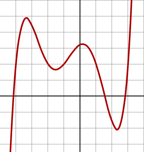 In the Zariski topology on \(\mathbb{A}^2\), closed sets are algebraic sets — zero loci of polynomials. Here the zero locus of a quintic polynomial is a closed set; open sets are complements of such curves, far coarser than the classical Euclidean topology.
Definition (Irreducibility). An algebraic set \(X\) is irreducible if it cannot be written as a union \(X = X_1 \cup X_2\) of two proper closed subsets. An irreducible algebraic set is called an affine variety.
\(V(I)\) is irreducible if and only if \(I(V(I))\) is a prime ideal. Every algebraic set decomposes uniquely into finitely many irreducible components.
1.2 Hilbert Basis Theorem
Theorem (Hilbert Basis Theorem). If \(k\) is a Noetherian ring, then \(k[x_1,\ldots,x_n]\) is Noetherian. In particular, \(k[x_1,\ldots,x_n]\) is Noetherian for any field \(k\).
Every algebraic set \(V(I)\) is cut out by finitely many polynomials — one can replace the ideal \(I\) by a finite generating set.
1.3 Nullstellensatz
The Nullstellensatz is the fundamental bridge between algebra and geometry.
Theorem (Weak Nullstellensatz). Let \(k\) be algebraically closed and \(I \subsetneq k[x_1,\ldots,x_n]\) a proper ideal. Then \(V(I) \neq \emptyset\).
Equivalently: the maximal ideals of \(k[x_1,\ldots,x_n]\) are exactly \(\mathfrak{m}_P = (x_1 - a_1,\ldots,x_n - a_n)\) for \(P = (a_1,\ldots,a_n) \in \mathbb{A}^n\).
Theorem (Strong Nullstellensatz). Let \(k\) be algebraically closed. For any ideal \(I \subset k[x_1,\ldots,x_n]\),
\[I(V(I)) = \sqrt{I},\]
where \(\sqrt{I} = \{ f \in k[x_1,\ldots,x_n] : f^m \in I \text{ for some } m \geq 1 \}\) is the radical of \(I\).
To show \(f \in I(V(I)) \Rightarrow f^m \in I\): introduce a new variable \(t\) and observe that \(V(I \cup \{1 - tf\}) = \emptyset\). By the Weak Nullstellensatz, \(1 \in \langle I, 1-tf \rangle\) in \(k[x_1,\ldots,x_n,t]\). Clearing \(t\) yields \(f^m \in I\).
1.4 The Radical Ideal Bijection
Definition (Ideal of a Set). For \(X \subset \mathbb{A}^n\), define
\[I(X) = \{ f \in k[x_1,\ldots,x_n] : f(P) = 0 \text{ for all } P \in X \}.\]
\(I(X)\) is always a radical ideal.
Theorem (Order-Reversing Bijection). Over an algebraically closed field \(k\), the maps \(V\) and \(I\) establish an inclusion-reversing bijection:
\[\left\{ \text{radical ideals of } k[x_1,\ldots,x_n] \right\} \longleftrightarrow \left\{ \text{algebraic sets in } \mathbb{A}^n \right\}\]
\[I \longmapsto V(I), \qquad X \longmapsto I(X).\]
Under this bijection: prime ideals correspond to irreducible varieties; maximal ideals correspond to points.
In \(\mathbb{A}^2\): \(I = (y - x^2)\) is prime, so \(V(I)\) is irreducible (the parabola). The ideal \((x,y)\) is maximal, corresponding to the origin \((0,0)\).
2. Coordinate Rings and Morphisms
2.1 Coordinate Ring
Definition (Coordinate Ring). For an affine variety \(X = V(I) \subset \mathbb{A}^n\), the coordinate ring of \(X\) is
\[k[X] = k[x_1,\ldots,x_n] / I(X).\]
Elements of \(k[X]\) are polynomial functions \(X \to k\). Two polynomials define the same function on \(X\) iff their difference vanishes on \(X\), i.e., lies in \(I(X)\).
Since \(I(X)\) is a radical ideal, \(k[X]\) is a reduced ring (no nonzero nilpotents). Since \(I(X)\) is prime when \(X\) is irreducible, \(k[X]\) is an integral domain for affine varieties.
2.2 Regular Functions and Morphisms
Definition (Regular Map). A map \(\phi: X \to Y\) between affine varieties (with \(Y \subset \mathbb{A}^m\)) is a regular map (or morphism) if it is the restriction of a polynomial map \(\mathbb{A}^n \to \mathbb{A}^m\): there exist \(f_1,\ldots,f_m \in k[x_1,\ldots,x_n]\) such that \(\phi(P) = (f_1(P),\ldots,f_m(P))\) for all \(P \in X\).
Regular maps are continuous in the Zariski topology: the preimage of a closed set is closed.
2.3 Pullback and Categorical Equivalence
Definition (Pullback). For a regular map \(\phi: X \to Y\), the pullback is the \(k\)-algebra homomorphism
\[\phi^*: k[Y] \to k[X], \qquad (\phi^* g)(P) = g(\phi(P)).\]
Theorem (Contravariant Equivalence). The functor \(X \mapsto k[X]\), \(\phi \mapsto \phi^*\) establishes a contravariant equivalence of categories:
\[\left\{ \text{affine varieties over } k \right\}^{\mathrm{op}} \simeq \left\{ \text{finitely generated reduced } k\text{-algebras} \right\}.\]
Morphisms of varieties correspond to \(k\)-algebra homomorphisms. Isomorphisms of varieties correspond to \(k\)-algebra isomorphisms.
The hyperbola \(V(xy-1) \subset \mathbb{A}^2\) has \(k[V(xy-1)] \cong k[x,x^{-1}]\), which is not isomorphic to \(k[t]\) (the coordinate ring of \(\mathbb{A}^1\)), reflecting the fact that the hyperbola is not isomorphic to the line.
3. Rational Functions and Local Rings
3.1 Rational Function Field
Definition (Rational Function Field). For an irreducible affine variety \(X\), since \(k[X]\) is an integral domain, one forms its field of fractions:
\[k(X) = \mathrm{Frac}(k[X]) = \left\{ \frac{f}{g} : f, g \in k[X],\ g \neq 0 \right\}.\]
\(k(X)\) is called the function field or rational function field of \(X\). A rational function \(\phi \in k(X)\) is an element \(f/g\) defined on the open set \(X \setminus V(g)\).
3.2 Local Ring at a Point
Definition (Local Ring). For \(P \in X\), let \(\mathfrak{m}_P \subset k[X]\) be the maximal ideal of functions vanishing at \(P\). The local ring of \(X\) at \(P\) is the localization
\[\mathcal{O}_{X,P} = k[X]_{\mathfrak{m}_P} = \left\{ \frac{f}{g} \in k(X) : g(P) \neq 0 \right\}.\]
\(\mathcal{O}_{X,P}\) is a local ring with maximal ideal \(\mathfrak{m}_{X,P} = \{ f/g \in \mathcal{O}_{X,P} : f(P) = 0 \}\).
\(\mathcal{O}_{X,P}\) is the ring of rational functions that are defined (i.e., have no pole) in some neighborhood of \(P\). The residue field \(\mathcal{O}_{X,P}/\mathfrak{m}_{X,P} \cong k\) recovers evaluation at \(P\). This is the algebraic analogue of the stalk of the structure sheaf at \(P\).
4. Affine Plane Curves
4.1 Multiplicity and Tangent Lines
🔢 Fix \(k\) algebraically closed, and let \(C = V(f) \subset \mathbb{A}^2\) be an affine plane curve, where \(f \in k[x,y]\) is a nonconstant polynomial.
Definition (Multiplicity). Write \(f\) as a sum of homogeneous components:
\[f = f_m + f_{m+1} + \cdots\]
where \(f_j\) is homogeneous of degree \(j\) and \(f_m \neq 0\). The multiplicity of \(C\) at \(P\) (after translating \(P\) to the origin) is
\[\mathrm{mult}_P(C) = m.\]
\(\mathrm{mult}_P(C) = 1\) iff \(P\) is a smooth (nonsingular) point of \(C\). \(\mathrm{mult}_P(C) \geq 2\) iff \(P\) is a singular point. \(\mathrm{mult}_P(C) \geq m\) means the curve vanishes to order at least \(m\) at \(P\).
Definition (Tangent Lines). The tangent lines to \(C\) at \(P\) (with \(P\) translated to origin) are the irreducible factors of the leading form \(f_m\). A tangent line \(L\) has multiplicity \(r\) if \((L)^r \mid f_m\) but \((L)^{r+1} \nmid f_m\).
\(C = V(y^2 - x^2(x+1))\): at the origin, \(f_2 = y^2 - x^2 = (y-x)(y+x)\), so \(P\) is a node with two distinct tangent lines \(y = x\) and \(y = -x\). \(C = V(y^2 - x^3)\): at the origin, \(f_2 = y^2\), so \(P\) is a cusp with one tangent line \(y = 0\) of multiplicity 2.
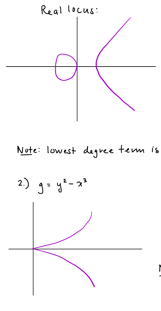 From Ullery’s Math 137 lecture notes. Top: a node — the nodal cubic \(y^2 = x^2(x+1)\) self-intersects at the origin, where two smooth branches cross with distinct tangent lines \(y = \pm x\) (the leading form \(y^2 - x^2\) factors into two distinct linear forms). Bottom: a cusp — \(y^2 = x^3\) has a single branch pinched to a point with one repeated tangent direction (leading form \(y^2 = (y)^2\) has repeated factor).
4.2 Branches at a Singularity
Informally, a branch of \(C\) at \(P\) corresponds to an irreducible component of the formal completion of \(\mathcal{O}_{C,P}\). A node has two distinct branches (two smooth arcs meeting transversely); a cusp has one branch (a single arc with a tangency). The number of branches can exceed \(\mathrm{mult}_P(C)\) in more complicated singularities.
The number of branches at \(P\) is not determined by \(\mathrm{mult}_P(C)\) alone — it depends on higher-order terms in the local equation.
5. Discrete Valuation Rings
5.1 Definition and Uniformizer
Definition (DVR). A discrete valuation ring (DVR) is a local principal ideal domain \(R\) that is not a field. Equivalently, \(R\) is a Noetherian local domain with a unique nonzero prime ideal.
A DVR has a unique maximal ideal \(\mathfrak{m} = (t)\) generated by a single element \(t\), called a uniformizer (or uniformizing parameter). Every nonzero element of \(R\) has the form \(u \cdot t^n\) for \(u \in R^\times\) and \(n \geq 0\), uniquely determined.
Definition (Discrete Valuation). Let \(R\) be a DVR with fraction field \(K\) and uniformizer \(t\). The discrete valuation associated to \(R\) is the map
\[v: K^\times \to \mathbb{Z}, \qquad v(u \cdot t^n) = n \text{ for } u \in R^\times.\]
Extended by convention to \(v(0) = +\infty\). This satisfies: 1. \(v(ab) = v(a) + v(b)\) (group homomorphism on \(K^\times\)). 2. \(v(a + b) \geq \min(v(a), v(b))\) (ultrametric inequality). 3. \(v\) is surjective onto \(\mathbb{Z}\).
5.2 The Valuation on a Curve
Let \(C\) be a smooth affine curve and \(P \in C\) a smooth point. The local ring \(\mathcal{O}_{C,P}\) is a DVR. Its maximal ideal \(\mathfrak{m}_P = (t)\) for some uniformizer \(t\) (e.g., a local coordinate vanishing simply at \(P\)). The valuation
\[v_P: k(C)^\times \to \mathbb{Z}\]
measures the order of vanishing (or pole order) of a rational function at \(P\): \(v_P(\phi) = n > 0\) means \(\phi\) has a zero of order \(n\) at \(P\); \(v_P(\phi) = -n < 0\) means \(\phi\) has a pole of order \(n\) at \(P\).
The valuation \(v_P\) captures the behavior of a rational function at the point \(P\) in the same way a complex analyst tracks zeros and poles. A regular function \(f \in k[C]\) satisfies \(v_P(f) \geq 0\) for all smooth \(P\).
5.3 DVRs and Smooth Points
Theorem. Let \(C\) be an irreducible curve with function field \(K = k(C)\). There is a canonical bijection:
\[\left\{ \text{smooth (nonsingular) points of } C \right\} \longleftrightarrow \left\{ \text{DVRs } R \subset K \text{ with } k \subset R \right\}.\]
Under this bijection, the smooth point \(P\) corresponds to the local ring \(\mathcal{O}_{C,P}\).
This bijection is the classical prototype for the modern definition of a scheme: points of a variety correspond to prime ideals (or valuation rings) of the function field. For smooth projective curves, every valuation of \(k(C)\) trivial on \(k\) arises from a unique point of \(C\).
6. Intersection Numbers
6.1 Fulton’s Definition
📐 Let \(C = V(f)\) and \(D = V(g)\) be affine plane curves in \(\mathbb{A}^2\), and let \(P \in \mathbb{A}^2\).
Definition (Intersection Number). The intersection number of \(C\) and \(D\) at \(P\) is
\[(C \cdot D)_P = \dim_k \mathcal{O}_{P} / (f, g),\]
where \(\mathcal{O}_P = \mathcal{O}_{\mathbb{A}^2, P}\) is the local ring of \(\mathbb{A}^2\) at \(P\) and \((f,g) \subset \mathcal{O}_P\) is the ideal generated by the images of \(f\) and \(g\).
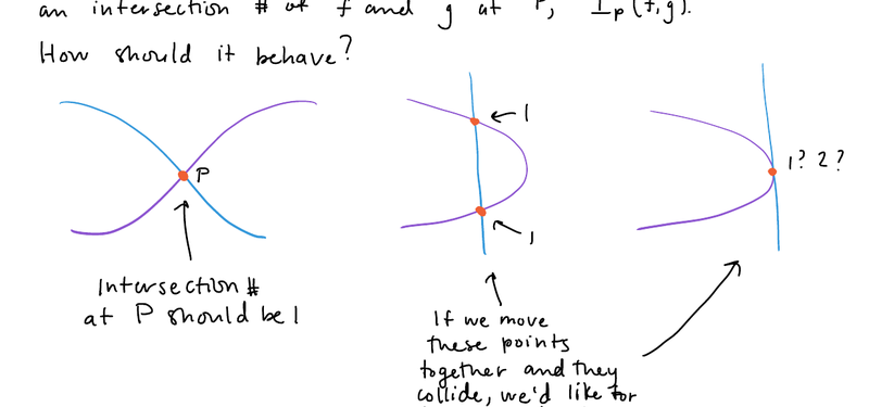 From Ullery’s Math 137 lecture notes on intersection numbers. Two curves crossing transversally at \(P\) should have intersection number 1; when one is tangent to the other, the two intersection points “merge” and the local count rises above 1. The definition \((C \cdot D)_P = \dim_k \mathcal{O}_P/(f,g)\) captures this contact order algebraically.
\((C \cdot D)_P\) counts — with multiplicity — how “tangentially” \(C\) and \(D\) meet at \(P\). Intuitively, it measures the dimension of the space of local conditions imposed by the two equations together at \(P\).
6.2 The Five Properties
The intersection number \((C \cdot D)_P\) is the unique function satisfying:
| # | Property | Statement |
|---|---|---|
| 1 | Finiteness | \((C \cdot D)_P < \infty\) iff \(C\) and \(D\) have no common component through \(P\). |
| 2 | Symmetry | \((C \cdot D)_P = (D \cdot C)_P\). |
| 3 | Positivity | \((C \cdot D)_P \geq 0\), with \((C \cdot D)_P = 0\) iff \(P \notin C \cap D\). |
| 4 | Additivity | \((C_1 C_2 \cdot D)_P = (C_1 \cdot D)_P + (C_2 \cdot D)_P\) when \(C = V(f_1 f_2)\). |
| 5 | Invariance | \((C \cdot D)_P\) is unchanged by a linear change of coordinates. |
An additional key property is that if \(P\) is a smooth point of both \(C\) and \(D\) and \(C, D\) meet transversally at \(P\) (distinct tangent lines), then \((C \cdot D)_P = 1\).
6.3 Key Example
Let \(C = V(f)\) be a plane curve of degree \(d\) and \(L\) a line not tangent to \(C\) at \(P\). Then \((C \cdot L)_P = \mathrm{mult}_P(C)\). In particular, a smooth point \(P \in C\) meets a generic line \(L\) transversally: \((C \cdot L)_P = 1\).
The parabola \(C = V(y - x^2)\) meets the \(x\)-axis \(L = V(y)\) at the origin with \((C \cdot L)_0 = 2\): the line is tangent to the parabola, and the two “intersection points” collide.
7. Projective Space and Varieties
7.1 Projective Space
Definition (Projective Space). Projective \(n\)-space over \(k\) is
\[\mathbb{P}^n_k = \left( k^{n+1} \setminus \{0\} \right) / \sim, \qquad (a_0,\ldots,a_n) \sim (\lambda a_0,\ldots,\lambda a_n) \text{ for } \lambda \in k^\times.\]
A point is an equivalence class, written with homogeneous coordinates \([a_0 : a_1 : \cdots : a_n]\).
 \(\mathbb{P}^n\) as the space of lines through the origin in \(k^{n+1}\): two nonzero vectors are identified iff they are scalar multiples. Affine space \(\mathbb{A}^n\) embeds as the open chart \(\{a_0 \neq 0\}\); “points at infinity” fill in the complementary hyperplane \(\{a_0 = 0\} \cong \mathbb{P}^{n-1}\).
Projective space compactifies affine space by adding “points at infinity” in each direction. Over \(\mathbb{C}\), \(\mathbb{P}^1_{\mathbb{C}}\) is the Riemann sphere; \(\mathbb{P}^2_{\mathbb{C}}\) is the complex projective plane. Many theorems (Bézout, Riemann-Roch) require projective space for clean statements.
7.2 Projective Algebraic Sets
A polynomial \(F \in k[x_0,\ldots,x_n]\) does not define a function on \(\mathbb{P}^n\) (its value depends on the representative), but its vanishing is well-defined if \(F\) is homogeneous: \(F(\lambda x_0,\ldots,\lambda x_n) = \lambda^d F(x_0,\ldots,x_n)\).
Definition (Projective Algebraic Set). For homogeneous polynomials \(F_1,\ldots,F_r \in k[x_0,\ldots,x_n]\), the projective algebraic set is
\[V_+(F_1,\ldots,F_r) = \{ [a_0:\cdots:a_n] \in \mathbb{P}^n : F_i(a_0,\ldots,a_n) = 0 \text{ for all } i \}.\]
Definition (Homogeneous Ideal). An ideal \(I \subset k[x_0,\ldots,x_n]\) is homogeneous if it is generated by homogeneous polynomials. For a projective algebraic set \(X\), define
\[I_+(X) = \{ F \in k[x_0,\ldots,x_n] : F \text{ homogeneous}, F|_X = 0 \} \cup \{0\}.\]
Definition (Homogeneous Coordinate Ring). The homogeneous coordinate ring of \(X = V_+(I)\) is the graded ring
\[S(X) = k[x_0,\ldots,x_n] / I_+(X) = \bigoplus_{d \geq 0} S(X)_d.\]
\(S(X)\) is NOT the ring of regular functions on \(X\). Homogeneous elements of \(S(X)\) are not functions on \(X\) (unless degree 0). The correct function ring requires working in local affine patches.
7.3 Standard Affine Cover
For each \(i = 0,\ldots,n\), the standard affine chart is
\[U_i = \{ [a_0:\cdots:a_n] \in \mathbb{P}^n : a_i \neq 0 \} \cong \mathbb{A}^n,\]
via the homeomorphism \([a_0:\cdots:a_n] \mapsto \left(\frac{a_0}{a_i},\ldots,\widehat{\frac{a_i}{a_i}},\ldots,\frac{a_n}{a_i}\right)\).
The \(n+1\) charts \(\{U_i\}\) cover \(\mathbb{P}^n\), and \(\mathbb{P}^n\) is the “gluing” of these copies of \(\mathbb{A}^n\) along the transition maps.
8. Morphisms of Projective Varieties
8.1 Regular Maps
A map \(\phi: X \to \mathbb{P}^m\) from a projective variety \(X\) is regular (or regular in a neighborhood) if locally in each affine chart it is given by polynomials. In global terms, if \(\phi = [F_0:\cdots:F_m]\) for homogeneous polynomials \(F_i\) of the same degree with no common zero on \(X\), then \(\phi\) is a regular map.
8.2 Veronese Embedding
Definition (Veronese Embedding). The \(d\)-th Veronese embedding is
\[\nu_d: \mathbb{P}^n \hookrightarrow \mathbb{P}^N, \qquad N = \binom{n+d}{d} - 1,\]
defined by \([x_0:\cdots:x_n] \mapsto [\ldots : x_0^{i_0}\cdots x_n^{i_n} : \ldots]\) where the coordinates range over all monomials of degree \(d\) in \(n+1\) variables.
\(\nu_d\) embeds \(\mathbb{P}^n\) as a subvariety of \(\mathbb{P}^N\) such that hyperplane sections of the image correspond to degree-\(d\) hypersurfaces in \(\mathbb{P}^n\). The \(d=2\), \(n=1\) case embeds \(\mathbb{P}^1\) as a conic in \(\mathbb{P}^2\).
8.3 Segre Embedding
Definition (Segre Embedding). The Segre embedding is
\[\sigma: \mathbb{P}^m \times \mathbb{P}^n \hookrightarrow \mathbb{P}^{(m+1)(n+1)-1},\]
defined by \(([x_0:\cdots:x_m], [y_0:\cdots:y_n]) \mapsto [\ldots : x_i y_j : \ldots]\) where the coordinates are all products \(x_i y_j\).
\(\sigma\) realizes the product \(\mathbb{P}^m \times \mathbb{P}^n\) as a projective variety. The image is the set of rank-1 matrices in the space of \((m+1)\times(n+1)\) matrices, i.e., the Segre variety.
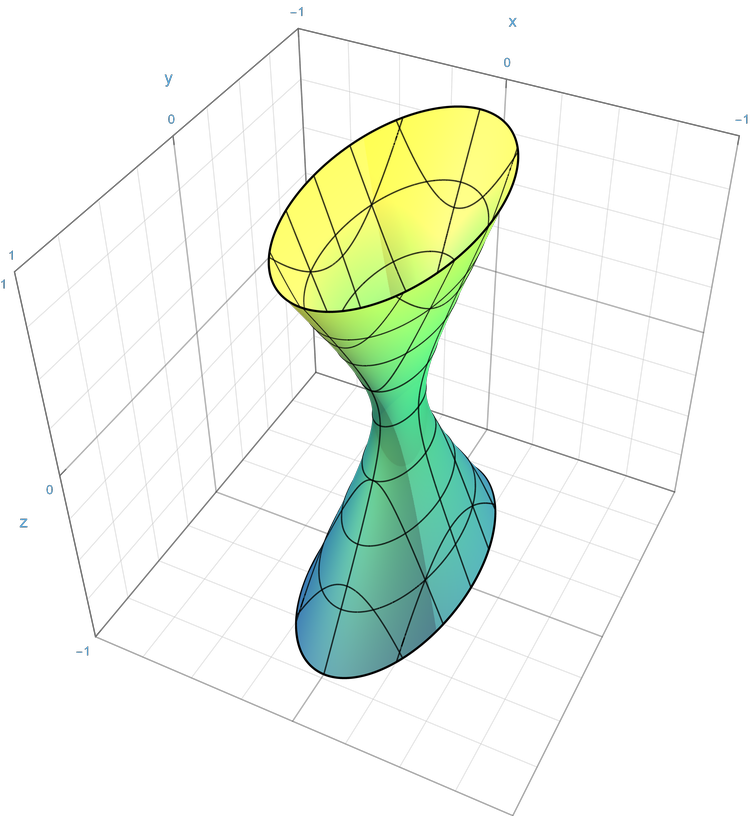 The Segre image \(\sigma(\mathbb{P}^1 \times \mathbb{P}^1) \subset \mathbb{P}^3\) is a smooth quadric surface — geometrically, a hyperboloid of one sheet. It carries two families of lines (rulings), corresponding to the two \(\mathbb{P}^1\) factors: fixing a point in one factor sweeps out a line in the other direction.
8.4 Quasiprojective Varieties
Definition (Quasiprojective Variety). A quasiprojective variety is an open subset of a projective variety (in the Zariski topology). Both affine varieties (open in their projective closure) and projective varieties are quasiprojective.
9. Projective Plane Curves
9.1 Degree and Homogeneous Polynomials
Definition (Projective Plane Curve). A projective plane curve of degree \(d\) is \(C = V_+(F) \subset \mathbb{P}^2\) where \(F \in k[x_0,x_1,x_2]\) is a nonzero homogeneous polynomial of degree \(d\).
The degree of the curve is the degree of its defining polynomial.
9.2 Projective Closure
Definition (Projective Closure). Let \(f \in k[x,y]\) be a polynomial of degree \(d\) defining an affine curve \(C_{\mathrm{aff}} = V(f) \subset \mathbb{A}^2\). The projective closure of \(C_{\mathrm{aff}}\) in \(\mathbb{P}^2\) is
\[\overline{C_{\mathrm{aff}}} = V_+(F) \subset \mathbb{P}^2,\]
where \(F(x_0,x_1,x_2) = x_0^d \cdot f(x_1/x_0, x_2/x_0)\) is the homogenization of \(f\).
The points at infinity of \(C_{\mathrm{aff}}\) are the points \(\overline{C_{\mathrm{aff}}} \setminus C_{\mathrm{aff}} = \overline{C_{\mathrm{aff}}} \cap \{x_0 = 0\}\).
The parabola \(V(y - x^2)\) in \(\mathbb{A}^2\) has homogenization \(F = x_0 x_2 - x_1^2\). Setting \(x_0 = 0\): \(-x_1^2 = 0\), so the only point at infinity is \([0:0:1]\). The projective closure is a smooth conic tangent to the line at infinity.
9.3 Genus Formula
Theorem (Genus of a Smooth Plane Curve). If \(C \subset \mathbb{P}^2\) is a smooth projective plane curve of degree \(d\), then the geometric genus of \(C\) is
\[g(C) = \binom{d-1}{2} = \frac{(d-1)(d-2)}{2}.\]
Notable values: \(d=1\) (line): \(g=0\); \(d=2\) (conic): \(g=0\); \(d=3\) (cubic/elliptic curve): \(g=1\); \(d=4\) (quartic): \(g=3\).
The genus formula is a special case of the adjunction formula in surface theory. For singular curves, one must subtract a correction for each singularity: \(g = \binom{d-1}{2} - \sum_P \delta_P\), where \(\delta_P\) is the delta invariant of the singularity at \(P\).
10. Linear Systems
10.1 Divisors on a Curve
Definition (Weil Divisor). On a smooth projective curve \(C\), a divisor is a formal finite \(\mathbb{Z}\)-linear combination of points:
\[D = \sum_{P \in C} n_P \cdot P, \qquad n_P \in \mathbb{Z},\ n_P = 0 \text{ for all but finitely many } P.\]
The degree of \(D\) is \(\deg D = \sum_P n_P\). A divisor \(D\) is effective (written \(D \geq 0\)) if \(n_P \geq 0\) for all \(P\).
Definition (Principal Divisor). For \(\phi \in k(C)^\times\), the principal divisor is
\[(\phi) = \sum_{P \in C} v_P(\phi) \cdot P.\]
Two divisors \(D\) and \(D'\) are linearly equivalent (\(D \sim D'\)) if \(D - D' = (\phi)\) for some \(\phi \in k(C)^\times\).
10.2 Complete Linear System
Definition (Complete Linear System). For a divisor \(D\) on a smooth projective curve \(C\), the complete linear system of \(D\) is
\[|D| = \{ D' \geq 0 : D' \sim D \} = \mathbb{P}(L(D)),\]
where \(L(D) = H^0(C, \mathcal{O}(D)) = \{ \phi \in k(C)^\times : (\phi) + D \geq 0 \} \cup \{0\}\) is the Riemann-Roch space of \(D\). Thus \(|D|\) is a projective space of dimension \(\ell(D) - 1\), where \(\ell(D) = \dim_k L(D)\).
Definition (Base Locus). The base locus of \(|D|\) is the set of points \(P\) lying in every divisor of \(|D|\):
\[\mathrm{Bs}(|D|) = \bigcap_{D' \in |D|} \mathrm{Supp}(D').\]
If \(\mathrm{Bs}(|D|) = \emptyset\), the linear system is base-point-free.
10.3 The Map to Projective Space
Definition (Map Defined by a Linear System). A base-point-free complete linear system \(|D|\) with \(\ell(D) = N+1\) determines a regular map
\[\phi_D: C \to \mathbb{P}^N, \qquad P \mapsto [\phi_0(P) : \cdots : \phi_N(P)],\]
where \(\phi_0,\ldots,\phi_N\) is any basis for \(L(D)\).
Definition (Very Ample). A divisor \(D\) is very ample if \(\phi_D: C \hookrightarrow \mathbb{P}^N\) is an embedding (injective with injective derivative). The linear system \(|D|\) is very ample if \(D\) is very ample.
Very ampleness means \(D\) provides enough functions to distinguish all points and tangent directions on \(C\) — it embeds \(C\) as a projective curve. Base-point-free means \(D\) at least defines a morphism (no “undefined” points).
11. Bezout’s Theorem
11.1 Statement
🔑 Theorem (Bézout). Let \(C = V_+(F)\) and \(D = V_+(G)\) be projective plane curves of degrees \(d = \deg F\) and \(e = \deg G\). If \(C\) and \(D\) have no common irreducible component, then
\[\sum_{P \in \mathbb{P}^2} (C \cdot D)_P = d \cdot e.\]
The total intersection count, with multiplicity, equals \(de\). The sum is finite since \(C \cap D\) is a finite set.
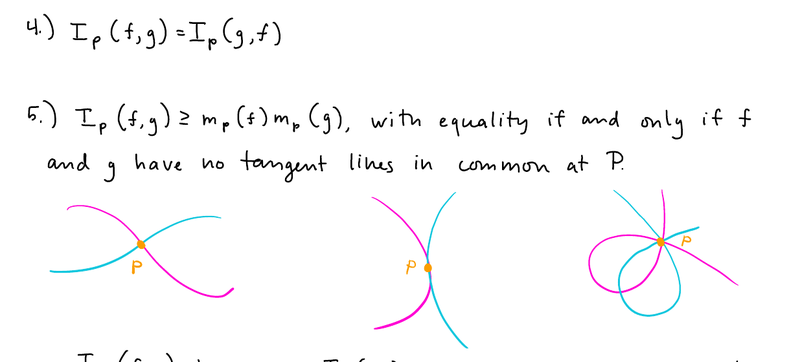 From Ullery’s Math 137 lecture notes. Three cases illustrating local intersection multiplicities: (left) transverse crossing, \(I_P = 1\); (middle) tangency, \(I_P > 1\); (right) a product of two curves each of degree 2 meeting, \(I_P = 2 \cdot 2 = 4\). Bézout’s theorem says these local multiplicities sum to \(\deg C \cdot \deg D\) over all points in \(\mathbb{P}^2\).
11.2 Proof Sketch
The key insight is that the intersection number is: 1. Additive in each argument: \((C_1 C_2 \cdot D)_P = (C_1 \cdot D)_P + (C_2 \cdot D)_P\). 2. Computable for a line: a line \(L\) meets a degree-\(d\) curve \(C\) at points summing to total intersection number \(d\) (by Bézout for curves and lines, proved by analyzing the restriction of \(F\) to \(L \cong \mathbb{P}^1\), which is a degree-\(d\) polynomial with exactly \(d\) roots counted with multiplicity).
For the general case, one argues that \(\sum_P (C \cdot D)_P\) depends only on \(\deg C\) and \(\deg D\). Fix a generic line \(L\): deform \(D\) linearly to \(L^e\) (a product of \(e\) lines) using a pencil in \(|D|\). Additivity gives \(\sum_P (C \cdot L^e)_P = e \cdot \sum_P (C \cdot L)_P = e \cdot d\).
Over \(\mathbb{A}^2\), the theorem fails: two parallel lines have degree \(1\) each but do not intersect. The projective completion forces them to meet at the point at infinity.
11.3 Applications
Two distinct lines in \(\mathbb{P}^2\) meet in exactly \(1 \cdot 1 = 1\) point. Any two distinct lines meet (no parallel lines in \(\mathbb{P}^2\)).
A smooth conic \(C\) (degree 2) and a line \(L\) (degree 1) satisfy \((C \cdot L)_\text{total} = 2\). If \(L\) is tangent to \(C\) at \(P\), then \((C \cdot L)_P = 2\) and the line meets \(C\) at only one point (with multiplicity 2). If \(L\) is secant, it meets \(C\) in two distinct points each with multiplicity 1.
A smooth curve \(C\) of degree \(d\) and a tangent line \(L\) at a smooth point \(P\) satisfy \((C \cdot L)_P \geq 2\). Since \(\sum_Q (C \cdot L)_Q = d\), the remaining intersections contribute at most \(d - 2\), so \(L\) meets \(C\) in at most \(d-1\) other points. A smooth curve cannot meet its tangent line at more than \(d\) points in total, with the tangent point counting at least twice.
12. Abstract Varieties
12.1 Gluing Construction
Definition (Abstract Variety). An abstract variety over \(k\) is a topological space \(X\) with a covering \(\{U_i\}\) by open sets, each isomorphic (as a ringed space) to an affine variety, such that the transition maps \(U_i \cap U_j \to U_i\) are regular maps.
More precisely: one specifies a collection of affine varieties \(\{V_i\}\), open subsets \(V_{ij} \subset V_i\), and isomorphisms \(\phi_{ij}: V_{ij} \xrightarrow{\sim} V_{ji}\) satisfying the cocycle condition \(\phi_{ki} = \phi_{kj} \circ \phi_{ji}\) on \(V_{ij} \cap V_{ik}\).
An abstract variety is separated if the diagonal \(\Delta_X \subset X \times X\) is closed. This is the algebro-geometric analogue of the Hausdorff condition and is automatically satisfied by quasiprojective varieties.
12.2 Function Field as Birational Invariant
Definition (Function Field of Abstract Variety). For an irreducible abstract variety \(X\), the function field \(k(X)\) is defined by taking any affine open subset \(U \subset X\): \(k(X) = k(U)\). This is independent of the choice of \(U\) (up to canonical isomorphism).
Birational geometry studies varieties up to isomorphism on dense open subsets. The function field \(k(X)\) completely characterizes the birational equivalence class of \(X\): two irreducible varieties \(X\) and \(Y\) are birationally equivalent iff \(k(X) \cong k(Y)\) as field extensions of \(k\).
Fact. \(\mathbb{P}^n\) as abstract variety is the gluing of \(n+1\) copies \(U_i \cong \mathbb{A}^n\) along transition maps \(U_i \cap U_j \cong \mathbb{A}^n \setminus V(x_i) \to U_j \cap U_i\) given by the rational maps \(x_k \mapsto x_k/x_j\).
13. Rational Maps and Dimension
13.1 Rational Maps
Definition (Rational Map). A rational map \(f: X \dashrightarrow Y\) between irreducible varieties is an equivalence class of pairs \((U, f_U)\) where \(U \subset X\) is a nonempty open set and \(f_U: U \to Y\) is a regular map, with two pairs equivalent if they agree on the intersection of their domains.
The domain of definition of \(f\) is the largest open set on which \(f\) is regular. The complement of the domain is the indeterminacy locus, a closed subset of dimension \(\leq \dim X - 2\) (for smooth \(X\)).
Definition (Dominant). A rational map \(f: X \dashrightarrow Y\) is dominant if its image is Zariski-dense in \(Y\).
 Stereographic projection is the prototypical example of a rational map that is not everywhere defined: projecting from the “north pole” \(N\) of the unit circle to \(\mathbb{P}^1\) gives a birational equivalence \(C \dashrightarrow \mathbb{P}^1\), undefined at \(N\) itself. This models projection from a point on a conic, showing that all smooth conics are birationally equivalent to \(\mathbb{P}^1\).
13.2 Birational Equivalence
Definition (Birational Equivalence). Irreducible varieties \(X\) and \(Y\) are birationally equivalent if there exist dominant rational maps \(f: X \dashrightarrow Y\) and \(g: Y \dashrightarrow X\) that are inverse to each other on dense open subsets. Equivalently, \(k(X) \cong k(Y)\) as \(k\)-algebras.
For smooth projective curves, every birational equivalence is an isomorphism. This fails in higher dimensions: many non-isomorphic surfaces are birationally equivalent (e.g., all rational surfaces are birational to \(\mathbb{P}^2\)).
13.3 Dimension
Definition (Dimension). The dimension of an irreducible variety \(X\) is the transcendence degree of its function field over \(k\):
\[\dim X = \mathrm{trdeg}_k \, k(X).\]
Equivalently: the length \(n\) of the longest chain of irreducible closed subsets \(\emptyset \neq Z_0 \subsetneq Z_1 \subsetneq \cdots \subsetneq Z_n = X\).
Notable values: \(\dim \mathbb{A}^n = \dim \mathbb{P}^n = n\); \(\dim V(f) = n-1\) for a hypersurface \(V(f) \subset \mathbb{A}^n\) with \(f\) irreducible.
13.4 Fiber Dimension Theorem
Theorem (Fiber Dimension Theorem). Let \(f: X \to Y\) be a dominant regular map of irreducible varieties. Then:
- For every point \(y \in f(X)\): \(\dim f^{-1}(y) \geq \dim X - \dim Y\).
- There exists a nonempty open set \(U \subset Y\) such that for all \(y \in U \cap f(X)\): \(\dim f^{-1}(y) = \dim X - \dim Y\).
The “generic fiber” has the expected codimension \(\dim X - \dim Y\). Special fibers can only be larger, never smaller. This is the algebraic geometry analogue of the rank-nullity theorem.
14. Blowing Up
14.1 Blow-up of a Point
🔧 Let \(P \in X\) be a point on a surface (a 2-dimensional variety). The blow-up of \(X\) at \(P\) is a variety \(\widetilde{X} = \mathrm{Bl}_P X\) together with a morphism \(\pi: \widetilde{X} \to X\) such that:
- \(\pi^{-1}(P) = E \cong \mathbb{P}^1\) (the exceptional divisor).
- \(\pi|_{\widetilde{X} \setminus E}: \widetilde{X} \setminus E \xrightarrow{\sim} X \setminus \{P\}\) is an isomorphism.
Local construction. In \(\mathbb{A}^2\) with coordinates \((x,y)\) and \(P = (0,0)\):
\[\mathrm{Bl}_0 \mathbb{A}^2 = \overline{\{((x,y), [u:v]) \in \mathbb{A}^2 \times \mathbb{P}^1 : xv = yu\}} \subset \mathbb{A}^2 \times \mathbb{P}^1.\]
The condition \(xv = yu\) says \((x,y)\) and \([u:v]\) point in the same direction. On the chart \(U_u = \{u \neq 0\}\): set \(u = 1\), coordinates \((x, v/u = y/x)\); on \(U_v = \{v \neq 0\}\): set \(v = 1\), coordinates \((u/v = x/y, y)\).
 From Ullery’s Math 137 lecture notes. The blow-up replaces the singular point \(P\) by a \(\mathbb{P}^1\) parametrizing all tangent directions at \(P\). The two branches of a node — which were merged at \(P\) — become separated in the blow-up, each meeting the exceptional divisor \(E \cong \mathbb{P}^1\) at a distinct direction.
14.2 Exceptional Divisor and Strict Transform
Definition (Exceptional Divisor). The fiber \(E = \pi^{-1}(P) \cong \mathbb{P}^1\) is the exceptional divisor. Geometrically, \(E\) parametrizes the directions of lines through \(P\): a point \([u:v] \in E\) corresponds to the limiting direction of approach to \(P\) along the slope \(v/u\).
Definition (Strict Transform). Let \(C \subset X\) be a curve through \(P\). The strict transform (or proper transform) \(\tilde{C} \subset \widetilde{X}\) is the closure of \(\pi^{-1}(C \setminus \{P\})\) in \(\widetilde{X}\).
The total transform is \(\pi^{-1}(C) = \tilde{C} \cup (m \cdot E)\) where \(m = \mathrm{mult}_P(C)\).
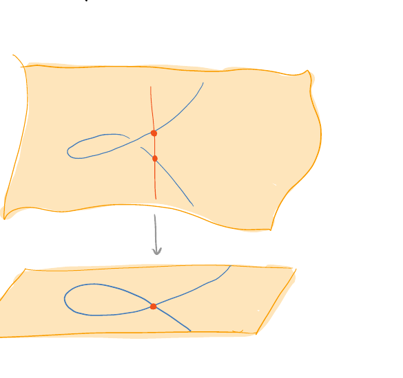
 From Ullery’s Math 137 lecture notes. In the local affine chart \(U\), the total preimage \(\pi^{-1}(C)\) of the nodal cubic is the union of the strict transform \(\tilde{C}\) (the non-compact branch passing through \(U\)) and the oval (the compact branch), meeting at the singular point marked in blue. The exceptional divisor \(E\) is the vertical white line in the center.
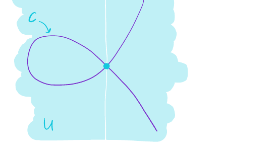
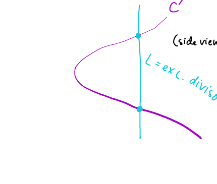 “Side view” from Ullery’s Math 137 notes. The strict transform \(\tilde{C}\) (purple) meets the exceptional divisor \(L = E\) (blue vertical line) at two distinct points — the two blue dots — corresponding to the two tangent directions \(y = \pm x\) at the node. A node requires exactly one blow-up to separate its two branches.
14.3 Resolution Examples
The origin is a node with \(\mathrm{mult}_0(C) = 2\) and two tangent lines \(y = \pm x\). After blowing up at the origin, the strict transform \(\tilde{C}\) is smooth. The two branches of \(C\) at the origin correspond to two distinct intersection points of \(\tilde{C}\) with the exceptional divisor \(E \cong \mathbb{P}^1\): the points \([1:1]\) and \([1:-1]\). The node has been resolved — the two branches are separated.
The origin is a cusp with \(\mathrm{mult}_0(C) = 2\) and one tangent line \(y = 0\) (with multiplicity 2). After blowing up, the strict transform \(\tilde{C}\) meets \(E\) at \([1:0]\) (only one point). On the chart \(U_u\): substituting \(y = xv\) gives \(x^2 v^2 - x^3 = x^2(v^2 - x) = 0\), so \(\tilde{C}\) is \(V(v^2 - x)\) in coordinates \((x,v)\) — a smooth parabola. The cusp is resolved in a single blow-up.
More complicated singularities (e.g., higher-order cusps) require iterated blow-ups. By Hironaka’s theorem (char 0), every algebraic variety admits a resolution of singularities by a finite sequence of blow-ups along smooth centers. The process terminates.
References
| Reference Name | Brief Summary | Link to Reference |
|---|---|---|
| Fulton, Algebraic Curves | The primary textbook for Harvard Math 137; covers algebraic sets, coordinate rings, local rings, DVRs, intersection numbers, Bézout’s theorem through a classical algebro-geometric lens. | http://www.math.lsa.umich.edu/~wfulton/CurveBook.pdf |
| Ullery, Math 137 Lecture Notes (Harvard) | 24-lecture undergraduate course notes following Fulton; primary source for this note’s organization and coverage. | https://people.math.harvard.edu/~bullery/math137/ |
| Ullery, Math 137 Lecture Notes (Emory mirror) | Alternate accessible mirror of the 24 lecture PDFs for Math 137. | http://math.emory.edu/~bullery/math137notes/index.html |
| Shafarevich, Basic Algebraic Geometry, Vol. 1 | Comprehensive reference for projective varieties, rational maps, dimension, and birational geometry; classical geometric flavor. | https://link.springer.com/book/9783642579080 |
| Reid, Undergraduate Algebraic Geometry | Accessible introduction with strong geometric intuition; good on plane curves, singularities, and blow-ups. | https://homepages.warwick.ac.uk/staff/Miles.Reid/MA4A5/UAG.pdf |
| Landesman, Math 137 Notes (Harris course) | Undergraduate algebraic geometry notes from a Harvard Math 137 offering with Joe Harris; complementary perspective. | https://people.math.harvard.edu/~landesman/assets/harris-undergrad-algebraic-geometry-notes.pdf |
| Zhang, Algebraic Curves Course Notes | Bath MA40188 course notes on algebraic curves; covers Nullstellensatz, coordinate rings, and function fields. | https://ziyuzhang.github.io/ma40188/Lecture_Notes_Long.pdf |
| Vakil, Foundations of Algebraic Geometry (Blow-ups) | Stanford FOAG classes 49-50 on blow-ups, exceptional divisors, and strict transforms. | https://math.stanford.edu/~vakil/0506-216/216class4950.pdf |
| Wikipedia: Bézout’s Theorem | Concise statement, proof outlines, and applications of Bézout’s theorem in algebraic geometry. | https://en.wikipedia.org/wiki/B%C3%A9zout%27s_theorem |
| Wikipedia: Discrete Valuation Ring | Definition, uniformizer, valuation, and connection to smooth points on curves. | https://en.wikipedia.org/wiki/Discrete_valuation_ring |
| Wikipedia: Linear System of Divisors | Complete linear systems, base locus, very ample divisors, and maps to projective space. | https://en.wikipedia.org/wiki/Linear_system_of_divisors |