Linear Attention, Chunkwise Training, and Neural Memory
Table of Contents
- 1. Introduction: Beyond Quadratic Compute and Linear Memory
- 2. Linear Attention: Removing Softmax
- 3. Training Efficiency Challenges
- 4. Chunkwise-Parallel Form
- 5. Decay and Gating Mechanisms
- 6. Neural Memory Perspective
- 7. References
1. Introduction: Beyond Quadratic Compute and Linear Memory
Standard softmax attention (see companion note standard-attention.md) operates with \(O(T^2 d_k)\) time and \(O(T^2)\) memory per layer, where \(T\) is the sequence length. During training this is managed by FlashAttention-style tiling, but during autoregressive inference a separate bottleneck emerges: the KV cache, which stores all \(T\) key and value vectors seen so far and grows as \(O(T \cdot (d_k + d_v))\) per layer. For a model with \(L\) layers, a sequence of length \(T = 128\text{k}\), and \(d_k = d_v = 128\), this is tens of gigabytes per forward pass — limiting the batch size and thus throughput.
This note addresses the family of architectures that replace softmax attention with a computation that:
- Maintains a state matrix of fixed size \(d_k \times d_v\) regardless of \(T\), eliminating KV-cache growth.
- Is expressible as a recurrence, enabling \(O(1)\) inference-time memory per layer.
- Admits a chunkwise-parallel training algorithm that recovers near-full GPU utilization while remaining mathematically equivalent to the recurrence.
We derive all recurrences from first principles, compare the decay and gating variants introduced by RetNet, Mamba-2, GLA, and RWKV, and close with the neural memory / fast weight programmer interpretation that places linear attention in a long line of associative memory research.
Notation. Scalars are italic (\(t\), \(\gamma\), \(\beta\)), vectors are bold (\(\mathbf{q}_t\), \(\mathbf{k}_t\), \(\mathbf{v}_t\)), and matrices are bold uppercase (\(S_t\), \(Q_i\), \(K_i\)). The sequence length is \(T\), chunk size is \(C\), key/query dimension is \(d_k\), and value dimension is \(d_v\). The outer product of column vectors \(\mathbf{a} \in \mathbb{R}^m\) and \(\mathbf{b} \in \mathbb{R}^n\) is denoted \(\mathbf{a} \mathbf{b}^\top \in \mathbb{R}^{m \times n}\); for row vectors \(\mathbf{k}_t \in \mathbb{R}^{1 \times d_k}\) we write \(\mathbf{k}_t^\top \mathbf{v}_t \in \mathbb{R}^{d_k \times d_v}\). We treat all token vectors as row vectors throughout to align with convention in the literature.
2. Linear Attention: Removing Softmax
2.1 Factored Dot-Product Attention
Recall standard causal (autoregressive) attention. For token \(t\), the output is:
\[\mathbf{o}_t = \frac{\sum_{j=1}^{t} \exp(\mathbf{q}_t \mathbf{k}_j^\top / \sqrt{d_k})\, \mathbf{v}_j}{\sum_{j=1}^{t} \exp(\mathbf{q}_t \mathbf{k}_j^\top / \sqrt{d_k})}\]
The softmax nonlinearity prevents factorization: because the normalization denominator couples all \(j\), one cannot separate the sum over \(j\) from the query \(\mathbf{q}_t\).
Katharopoulos et al. (2020) propose replacing the kernel \(\exp(\mathbf{q}\mathbf{k}^\top / \sqrt{d_k})\) with a factored similarity \(\phi(\mathbf{q})\phi(\mathbf{k})^\top\), where \(\phi : \mathbb{R}^{d_k} \to \mathbb{R}^r\) is a feature map. This gives:
\[\mathbf{o}_t = \frac{\sum_{j=1}^{t} \phi(\mathbf{q}_t)\phi(\mathbf{k}_j)^\top\, \mathbf{v}_j}{\sum_{j=1}^{t} \phi(\mathbf{q}_t)\phi(\mathbf{k}_j)^\top \cdot \mathbf{1}}\]
Since \(\phi(\mathbf{q}_t)\) does not depend on \(j\), it factors out of both numerator and denominator:
\[\mathbf{o}_t = \frac{\phi(\mathbf{q}_t) \left(\sum_{j=1}^{t} \phi(\mathbf{k}_j)^\top \mathbf{v}_j\right)}{\phi(\mathbf{q}_t) \left(\sum_{j=1}^{t} \phi(\mathbf{k}_j)^\top\right)}\]
The denominator is a scalar normalizer. In much of the subsequent literature — and throughout this note — the normalizer is dropped or absorbed, and the simplest feature map \(\phi(\mathbf{x}) = \mathbf{x}\) (identity) is used. This yields what is most commonly called linear attention:
\[\textcolor{#D35400}{\mathbf{o}_t} = \textcolor{#D35400}{\mathbf{q}_t} \sum_{j=1}^{t} \textcolor{#2E86C1}{\mathbf{k}_j}^\top \textcolor{#2E86C1}{\mathbf{v}_j}\]
This identity-feature-map form is the starting point for all recurrences below.
2.2 The State Matrix and Recurrence Relation
Define the state matrix at time \(t\) as the running sum of outer products:
📐 Definition (Linear Attention State). Let \(\mathbf{k}_j \in \mathbb{R}^{1 \times d_k}\) and \(\mathbf{v}_j \in \mathbb{R}^{1 \times d_v}\) be the key and value row vectors at position \(j\). The state matrix is:
\[\textcolor{#2E86C1}{S_t} = \sum_{j=1}^{t} \textcolor{#2E86C1}{\mathbf{k}_j}^\top \textcolor{#2E86C1}{\mathbf{v}_j} \in \mathbb{R}^{d_k \times d_v}\]
Each term \(\textcolor{#2E86C1}{\mathbf{k}_j}^\top \textcolor{#2E86C1}{\mathbf{v}_j}\) is a rank-1 outer product. The output of linear attention for token \(t\) is then:
\[\textcolor{#D35400}{\mathbf{o}_t} = \textcolor{#D35400}{\mathbf{q}_t} \textcolor{#2E86C1}{S_t} \in \mathbb{R}^{1 \times d_v}\]
From the definition of \(\textcolor{#2E86C1}{S_t}\), we immediately derive the recurrence:
\[\textcolor{#2E86C1}{S_t} = \textcolor{#2E86C1}{S_{t-1}} + \textcolor{#2E86C1}{\mathbf{k}_t}^\top \textcolor{#2E86C1}{\mathbf{v}_t}, \qquad \textcolor{#2E86C1}{S_0} = \mathbf{0}\]
This is a rank-1 update: the new state equals the old state plus a single outer product. The update costs \(O(d_k \cdot d_v)\) time and the output computation \(\textcolor{#D35400}{\mathbf{o}_t} = \textcolor{#D35400}{\mathbf{q}_t} \textcolor{#2E86C1}{S_t}\) costs the same — both are independent of \(T\).
2.3 Linear RNN Interpretation
The pair \((S_t, \mathbf{o}_t)\) defines a recurrent neural network whose hidden state is the matrix \(S_t \in \mathbb{R}^{d_k \times d_v}\):
\[S_t = S_{t-1} + \mathbf{k}_t^\top \mathbf{v}_t, \qquad \mathbf{o}_t = \mathbf{q}_t S_t\]
The transition is linear in \(S_{t-1}\) (the coefficient is the identity map), hence the name linear attention / linear RNN. This stands in contrast to LSTMs and GRUs, which have nonlinear gating in the state transition. The keys \(\mathbf{k}_t\) and values \(\mathbf{v}_t\) are the “write” operands and the query \(\mathbf{q}_t\) is the “read” operand — a clean read/write decomposition of memory.
Crucially, the hidden state \(S_t\) has dimension \(d_k \times d_v\) at every step, regardless of \(T\). During inference one need only store \(S_t\), not all past keys and values.
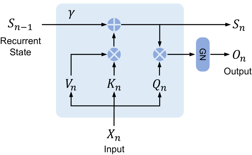 Figure 3b (Sun et al., 2023): The recurrent form of the retention mechanism. At each step the recurrent state \(S_{n-1}\) is scaled by the decay \(\gamma\), incremented by the outer product \(K_n^\top V_n\) (write), and then read by \(Q_n\) to produce output \(O_n\). This is exactly the linear attention recurrence \(S_t = \gamma S_{t-1} + \mathbf{k}_t^\top \mathbf{v}_t\), \(\mathbf{o}_t = \mathbf{q}_t S_t\), making the RNN structure of the state matrix explicit.
2.4 Memory Complexity Comparison
| Scheme | Inference memory per layer |
|---|---|
| Softmax attention (KV cache) | \(O(T \cdot (d_k + d_v))\) — grows with \(T\) |
| Linear attention (state matrix) | \(O(d_k \cdot d_v)\) — constant in \(T\) |
🔑 During inference, the linear attention state matrix costs \(O(d_k \cdot d_v)\) memory regardless of sequence length, eliminating the KV-cache growth bottleneck.
For typical values \(d_k = d_v = 128\), this is a matrix of \(128 \times 128 = 16{,}384\) floats (\(\approx 64\) KB per head) — fixed, no matter how long the sequence grows.
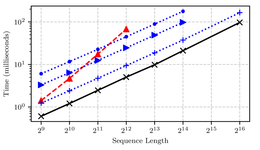 Figure 1 (Katharopoulos et al., 2020): Wall-clock time (ms) versus sequence length for softmax attention (blue, dashed, \(O(T^2)\) slope), linear attention (black solid, \(O(T)\) slope), and Reformer LSH variants (blue dotted). Linear attention’s time grows linearly with \(T\), while softmax attention grows quadratically — directly reflecting the constant-memory recurrence versus the KV-cache growth shown in the table above.
3. Training Efficiency Challenges
3.1 Sequential Recurrence Bottleneck
⚠️ The recurrence \(S_t = S_{t-1} + \mathbf{k}_t^\top \mathbf{v}_t\) is inherently sequential: \(S_t\) depends on \(S_{t-1}\), which depends on \(S_{t-2}\), and so on. During training, where all \(T\) tokens are available simultaneously, naive execution of this recurrence requires \(T\) sequential steps. This defeats the parallel computation advantage that made softmax attention fast to train via matrix multiplications on GPUs.
By contrast, standard softmax attention processes the full sequence as a single \(T \times T\) matrix multiply — all entries of \(Q K^\top\) are computed in parallel. The linear recurrence sacrifices this parallelism for the memory advantage.
3.2 Outer-Product Operations and GPU Utilization
Each state update \(S_t \leftarrow S_{t-1} + \mathbf{k}_t^\top \mathbf{v}_t\) involves a \(d_k \times d_v\) outer product. On a GPU, this is a rank-1 update to an \(O(d^2)\) matrix — a memory-bound operation. The arithmetic intensity (FLOPs per byte transferred) is too low to saturate the tensor cores designed for large matrix multiplies. Running \(T\) such updates sequentially compounds the problem: total wall time scales with \(T\) even though the total FLOPs are low.
3.3 IO Overhead from State Materialization
If one materializes the full state trajectory \(\{S_0, S_1, \ldots, S_T\}\) for backpropagation, the memory cost is \(O(T \cdot d_k \cdot d_v)\) — the very bottleneck linear attention was meant to avoid. The alternative is gradient checkpointing: recompute \(S_t\) from \(S_0\) during the backward pass, paying \(O(T)\) recomputation cost. Neither option is fully satisfactory for long sequences.
The chunkwise-parallel form in Section 4 resolves all three challenges simultaneously.
4. Chunkwise-Parallel Form
The key insight is that the linear recurrence can be re-expressed in a block form that separates within-chunk (parallel) from between-chunk (sequential) computation. The resulting algorithm — known as the chunkwise or chunkwise-recurrent form — is mathematically identical to the full recurrence; no approximation is involved.
4.1 Splitting into Chunks
Partition the \(T\) tokens into \(N = T/C\) non-overlapping chunks of size \(C\), where \(C\) divides \(T\). Chunk \(i\) contains positions \(\{(i-1)C + 1, \ldots, iC\}\). Denote the stacked query, key, and value matrices for chunk \(i\) as:
\[Q_i \in \mathbb{R}^{C \times d_k}, \quad K_i \in \mathbb{R}^{C \times d_k}, \quad V_i \in \mathbb{R}^{C \times d_v}\]
Let \(S_{i}^\text{end}\) denote the state at the end of chunk \(i\) (i.e., at position \(iC\)), and \(S_i^\text{start} = S_{i-1}^\text{end}\) the state entering chunk \(i\). Define \(S_0^\text{end} = \mathbf{0}\).
4.2 Intra-Chunk: Parallel Output Computation
Within chunk \(i\), each token \(t\) attends only to tokens within the same chunk that precede it (causal masking within the chunk). The output for the \(s\)-th token inside chunk \(i\) (local index \(s \in \{1, \ldots, C\}\)) from tokens within the same chunk is:
\[\mathbf{o}_s^\text{intra} = \sum_{j=1}^{s} \mathbf{q}_s \mathbf{k}_j^\top \mathbf{v}_j = \mathbf{q}_s \underbrace{\left(\sum_{j=1}^{s} \mathbf{k}_j^\top \mathbf{v}_j\right)}_{\text{partial state within chunk}}\]
In matrix form, stacking all \(C\) outputs:
\[O_i^\text{intra} = \underbrace{(Q_i K_i^\top \odot M)}_{\text{lower-triangular masked scores}} V_i \in \mathbb{R}^{C \times d_v}\]
where \(M \in \{0, 1\}^{C \times C}\) is a lower-triangular causal mask (\(M_{s,j} = 1\) iff \(s \geq j\)). This is a standard dense matrix multiply — GPU-friendly and fully parallel across all \(C \times C\) pairs.
4.3 Inter-Chunk: Recurrent State Passing
The state at the end of chunk \(i\) is:
\[S_i^\text{end} = S_{i-1}^\text{end} + K_i^\top V_i\]
where \(K_i^\top V_i = \sum_{s=1}^{C} \mathbf{k}_{(i-1)C+s}^\top \mathbf{v}_{(i-1)C+s}\) sums the \(C\) outer products in chunk \(i\). The computation \(K_i^\top V_i \in \mathbb{R}^{d_k \times d_v}\) is a matrix multiply of shape \((d_k \times C) \cdot (C \times d_v)\) — again GPU-friendly.
The recurrence \(S_i^\text{end} = S_{i-1}^\text{end} + K_i^\top V_i\) is sequential in \(i\), but now runs only \(N = T/C\) steps rather than \(T\) steps. For \(C = 64\), this reduces the sequential depth by a factor of 64.
4.4 Output Decomposition into Two Parts
Each token inside chunk \(i\) also receives contributions from all tokens in chunks \(0, 1, \ldots, i-1\) — captured by the state \(S_{i-1}^\text{end}\) entering chunk \(i\). The inter-chunk contribution for all tokens in chunk \(i\) is:
\[O_i^\text{inter} = Q_i \, S_{i-1}^\text{end} \in \mathbb{R}^{C \times d_v}\]
This is a single matrix multiply \((C \times d_k) \cdot (d_k \times d_v)\), again fully parallel.
The total output for chunk \(i\) is:
\[O_i = O_i^\text{inter} + O_i^\text{intra} = Q_i S_{i-1}^\text{end} + (Q_i K_i^\top \odot M) V_i\]
This decomposition is exact: it equals the output one would obtain by running the full token-level recurrence, with no approximation.
Proof sketch. For the \(s\)-th token in chunk \(i\) (absolute index \(t = (i-1)C + s\)):
\[\mathbf{o}_t = \mathbf{q}_t S_t = \mathbf{q}_t \left( S_{i-1}^\text{end} + \sum_{j=1}^{s} \mathbf{k}_{(i-1)C+j}^\top \mathbf{v}_{(i-1)C+j} \right) = \underbrace{\mathbf{q}_t S_{i-1}^\text{end}}_{\text{inter}} + \underbrace{\mathbf{q}_t \sum_{j=1}^{s} \mathbf{k}_j^\top \mathbf{v}_j}_{\text{intra}}\]
Stacking over \(s = 1, \ldots, C\) gives \(O_i = O_i^\text{inter} + O_i^\text{intra}\). \(\square\)
4.5 IO-Aware Implementation
The chunkwise form lends itself to a FlashAttention-style tiling strategy (used in FlashLinearAttention / GLA). The key observations are:
- The state \(S_i^\text{end} \in \mathbb{R}^{d_k \times d_v}\) is reused for \(O_i^\text{inter}\) of the next chunk. It fits in SRAM for typical head dimensions.
- The intra-chunk computation \((Q_i K_i^\top \odot M) V_i\) is a local \((C \times C)\) attention with \(C \ll T\), fitting the \(Q_i, K_i, V_i\) blocks in SRAM.
- The inter-chunk state update \(S_i \leftarrow S_{i-1} + K_i^\top V_i\) reduces to a single \((d_k \times C) \cdot (C \times d_v)\) GEMM per chunk.
By fusing all four operations (state update, \(O_i^\text{inter}\), masked intra-chunk attention, output accumulation) into a single kernel, HBM reads/writes are minimized. This is the approach of Yang et al.’s FlashLinearAttention algorithm.
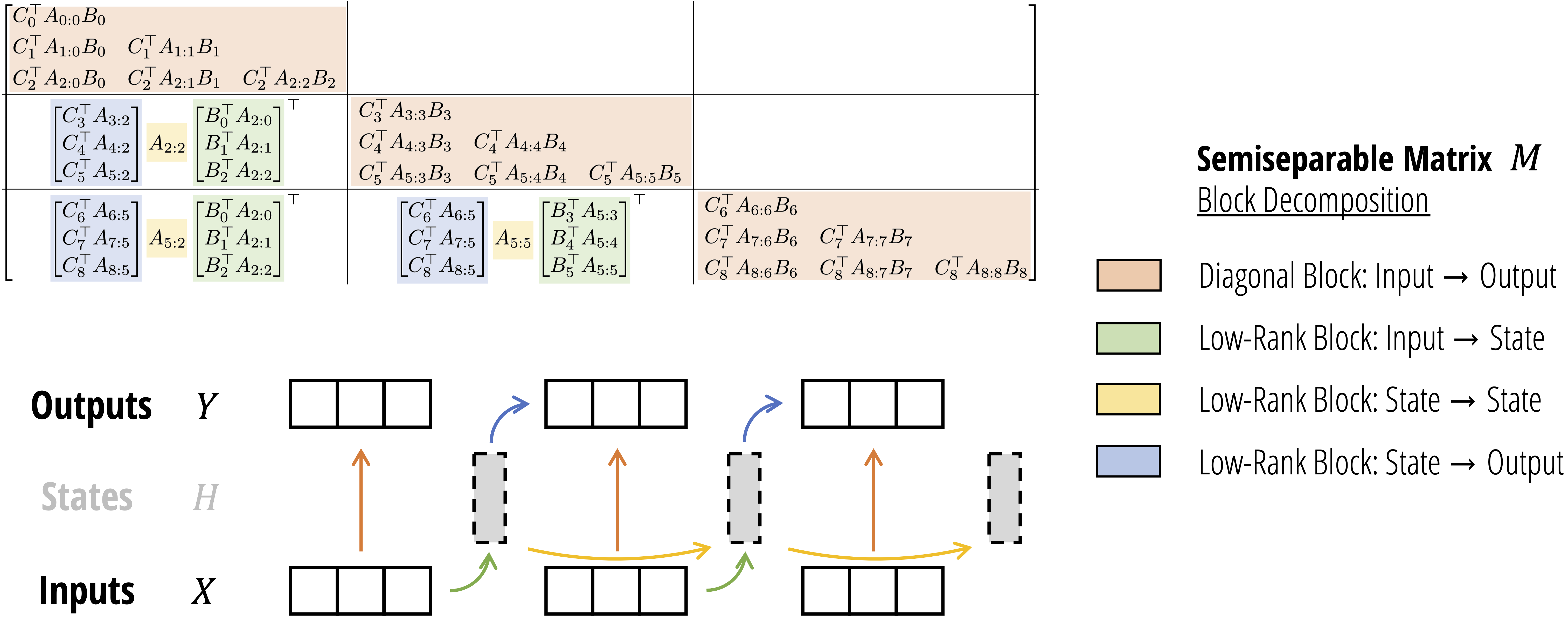 Figure (Dao & Gu, 2024): The SSD chunkwise algorithm. Top: the output matrix \(Y = MX\) where \(M\) is a semiseparable matrix, shown tiled into four block types — orange (diagonal intra-chunk, computed as masked attention), green (low-rank input-to-state), yellow (low-rank state-to-state recurrence), and blue (low-rank state-to-output). Bottom: the corresponding data-flow — inputs \(X\) are processed within each chunk (intra), states \(H\) accumulate across chunks (inter), and outputs \(Y\) combine both contributions. This decomposition is exactly the chunkwise form \(O_i = Q_i S_{i-1}^\text{end} + (Q_i K_i^\top \odot M)V_i\) derived above.
5. Decay and Gating Mechanisms
5.1 Motivation: Recency Bias and Bounded Memory
In pure linear attention, all past tokens contribute equally to the state \(S_t\): older outer products are never discounted. For long sequences this causes the state to be dominated by the earliest tokens, since contributions accumulate without bound. A decay factor \(\gamma \in (0, 1)\) multiplies the state at each step, exponentially downweighting older information and introducing a recency bias.
Algebraically, the state with decay satisfies:
\[S_t = \gamma S_{t-1} + \mathbf{k}_t^\top \mathbf{v}_t\]
Unrolling \(n\) steps: \(S_t = \sum_{j=1}^{t} \gamma^{t-j} \mathbf{k}_j^\top \mathbf{v}_j\). The contribution of token \(j\) decays exponentially as \(\gamma^{t-j}\), so the effective memory horizon is \(\approx (1-\gamma)^{-1}\) tokens.
5.2 Constant Scalar Decay: RetNet
Sun et al. (2023) introduced the Retentive Network (RetNet), in which the state transition uses a fixed scalar decay \(\gamma \in (0,1)\) combined with complex-valued rotary encodings. In the simplified scalar form:
📐 Definition (RetNet Retention). The retention state satisfies:
\[\textcolor{#2E86C1}{S_t} = \textcolor{#1E8449}{\gamma} \textcolor{#2E86C1}{S_{t-1}} + \textcolor{#2E86C1}{\mathbf{k}_t}^\top \textcolor{#2E86C1}{\mathbf{v}_t}, \qquad \textcolor{#D35400}{\mathbf{o}_t} = \textcolor{#D35400}{\mathbf{q}_t} \textcolor{#2E86C1}{S_t}\]
where \(\textcolor{#1E8449}{\gamma}\) is a head-specific constant (different heads use different decay values). The parallel form writes the full-sequence output as:
\[O = (Q K^\top \odot D) V\]
where \(D \in \mathbb{R}^{T \times T}\) is the decay mask with \(D_{t,j} = \gamma^{t-j}\) for \(t \geq j\) and \(0\) otherwise. RetNet assigns \(\gamma_h = 1 - 2^{-(5+h)}\) for head \(h\), giving a geometric spread of memory horizons across heads.
The chunkwise form of RetNet accumulates the decayed state at chunk boundaries. Letting \(B = C\) be chunk size and \(R_{i-1}\) the state entering chunk \(i\):
\[R_i = \gamma^C R_{i-1} + K_i^\top (V_i \odot \zeta_i)\]
where \(\zeta_i\) is a per-token decay weight within the chunk. The factor \(\gamma^C\) discounts the entire previous state by the chunk length.
💡 The constant \(\gamma\) is never updated at inference time — it is a fixed hyperparameter, not a learned function of the input. This is both its strength (no input-dependent overhead) and its weakness (the effective memory horizon is fixed and cannot adapt to content).
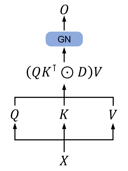 Figure 3a (Sun et al., 2023): The parallel representation of retention. Input \(X\) is projected to \(Q\), \(K\), \(V\); the output is \((QK^\top \odot D)V\) where \(D\) is the decay mask with \(D_{t,j} = \gamma^{t-j}\); GroupNorm (GN) normalizes the result. This is the training-time parallel form of the RetNet recurrence — a standard masked matrix multiply with a geometric decay mask in place of the usual binary causal mask.
5.3 Scalar Data-Dependent Decay: Mamba-2
Dao and Gu (2024) introduce the State Space Duality (SSD) framework in Mamba-2. The key architectural change is making the decay a scalar function of the input at each step:
📐 Definition (SSD Layer). The SSD recurrence is:
\[\textcolor{#2E86C1}{S_t} = \textcolor{#1E8449}{a_t} \textcolor{#2E86C1}{S_{t-1}} + \mathbf{b}_t^\top x_t, \qquad y_t = \mathbf{c}_t \textcolor{#2E86C1}{S_t}\]
where \(a_t \in \mathbb{R}\) is a scalar derived from input \(x_t\) (typically \(a_t = \sigma(w_a^\top x_t)\) for some learned vector \(w_a\)), and \(\mathbf{b}_t, \mathbf{c}_t\) are the data-dependent key and query analogues.
The scalar-times-identity constraint on \(A\) — that is, \(A_t = a_t I_{d_k}\) where \(I_{d_k}\) is the identity matrix — distinguishes SSD from earlier SSMs (which allow fully diagonal or even dense \(A_t\)). This constraint is what makes the connection to linear attention exact and enables a tensor-core-friendly chunkwise algorithm.
In attention notation with \(a_t = \textcolor{#1E8449}{\gamma_t}\) (data-dependent scalar decay):
\[\textcolor{#2E86C1}{S_t} = \textcolor{#1E8449}{\gamma_t} \textcolor{#2E86C1}{S_{t-1}} + \textcolor{#2E86C1}{\mathbf{k}_t}^\top \textcolor{#2E86C1}{\mathbf{v}_t}, \qquad \textcolor{#D35400}{\mathbf{o}_t} = \textcolor{#D35400}{\mathbf{q}_t} \textcolor{#2E86C1}{S_t}\]
The parallel (attention-form) dual constructs a lower-triangular matrix \(L \in \mathbb{R}^{T \times T}\):
\[L_{t,j} = \prod_{s=j+1}^{t} \gamma_s \quad (t \geq j), \qquad L_{t,j} = 0 \quad (t < j)\]
Then \(O = (L \odot Q K^\top) V\), which is a structured masked attention that generalizes RetNet’s geometric decay mask. 🔑 The scalar constraint on \(A_t\) is precisely what preserves the matrix-multiply structure in \(L\), keeping the chunkwise algorithm hardware-efficient.
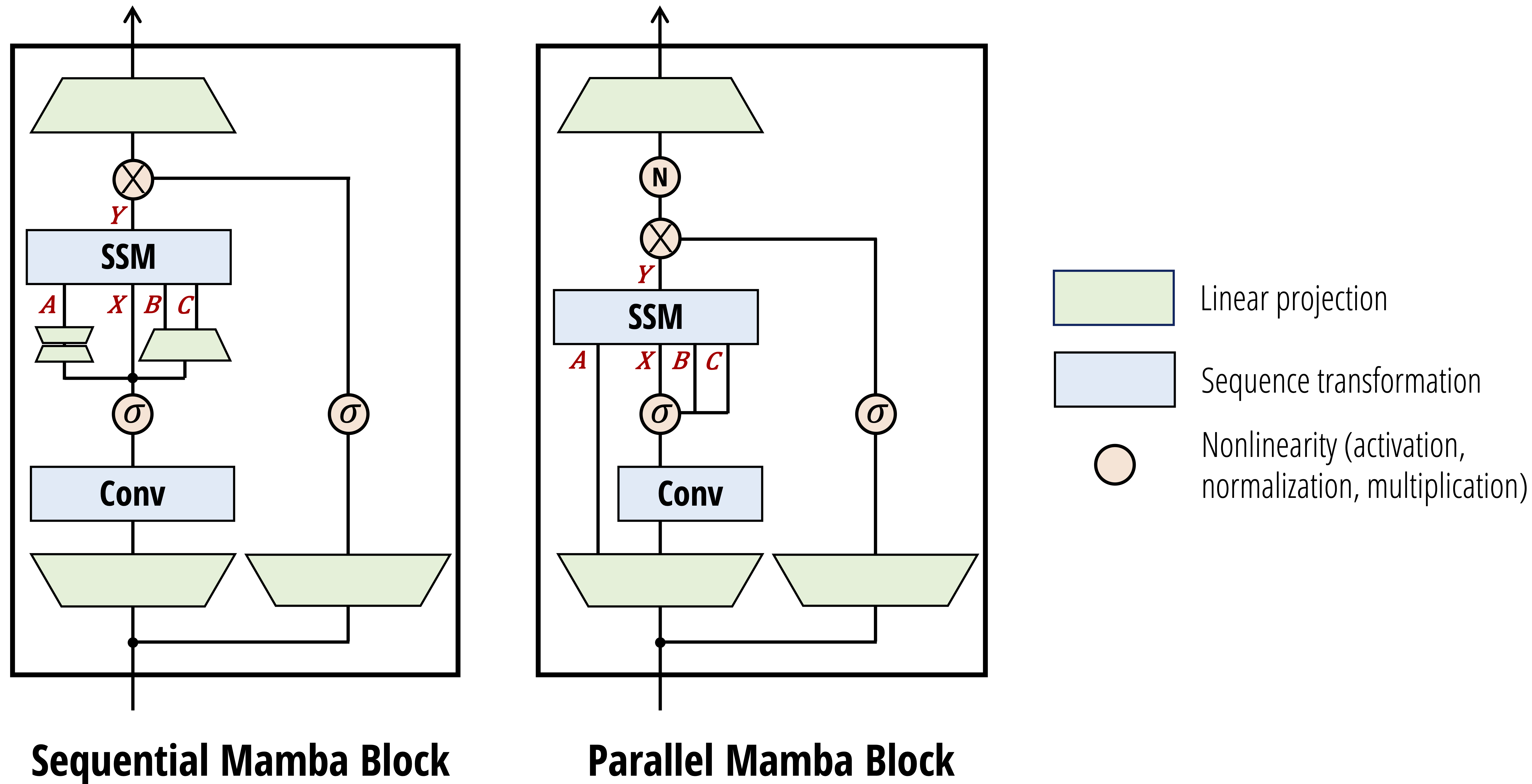 Figure (Dao & Gu, 2024): The Mamba-2 block in sequential (left) and parallel (right) forms. The SSM parameters \(A\) (scalar decay), \(X\) (input), \(B\) (key analogue), and \(C\) (query analogue) are produced by learned projections; the gating \(\sigma\) on the right branch creates the SiLU-gated output. The key architectural change from Mamba-1 is that \(A\), \(B\), \(C\) are now computed in parallel from the same input, making the block compatible with the tensor-parallel training setup required by the SSD chunkwise algorithm.
5.4 Vector Data-Dependent Gating: GLA
Yang et al. (2024) introduce Gated Linear Attention (GLA), which generalizes the scalar gate to a vector-valued gate while preserving the outer-product structure of the state update:
📐 Definition (GLA State Update). The GLA recurrence uses element-wise gates:
\[\textcolor{#2E86C1}{S_t} = (\textcolor{#1E8449}{\boldsymbol{\alpha}_t} \textcolor{#1E8449}{\boldsymbol{\beta}_t}^\top) \odot \textcolor{#2E86C1}{S_{t-1}} + \textcolor{#2E86C1}{\mathbf{k}_t}^\top \textcolor{#2E86C1}{\mathbf{v}_t}\]
where \(\textcolor{#1E8449}{\boldsymbol{\alpha}_t} \in \mathbb{R}^{d_k}\) and \(\textcolor{#1E8449}{\boldsymbol{\beta}_t} \in \mathbb{R}^{d_v}\) are data-dependent vectors, and \(\odot\) denotes element-wise (Hadamard) multiplication. The gate matrix \(\textcolor{#1E8449}{\boldsymbol{\alpha}_t} \textcolor{#1E8449}{\boldsymbol{\beta}_t}^\top \in \mathbb{R}^{d_k \times d_v}\) is rank-1, which is the crucial structural property.
💡 Why must the gate be rank-1? If the gate were an arbitrary matrix \(G_t \in \mathbb{R}^{d_k \times d_v}\), the state update \(G_t \odot S_{t-1}\) would break the outer-product recurrence: the chunkwise state \(K_i^\top V_i\) would no longer have a clean matrix-multiply form when propagated through the gate. The rank-1 factorization \(\boldsymbol{\alpha}_t \boldsymbol{\beta}_t^\top\) ensures the cumulative gate across a chunk is still an outer product, preserving the \((d_k \times C)(C \times d_v)\) GEMM structure in the FlashLinearAttention kernel.
Computing \(\boldsymbol{\alpha}_t\) and \(\boldsymbol{\beta}_t\) from input \(x_t\) via a learned linear map adds minimal overhead. GLA empirically outperforms RetNet and standard linear attention while achieving training speed competitive with FlashAttention-2.
RWKV-6 (Peng et al., 2024) uses a related vector gating scheme, applying data-dependent linear interpolation (ddlerp) to construct per-channel decay vectors, combined with LoRA-style low-rank adaptation for efficiency.
6. Neural Memory Perspective
6.1 Standard Attention as Associative Memory
Softmax attention can be viewed as a content-addressable memory (Hopfield network interpretation). The context stores \(T\) key-value pairs \(\{(\mathbf{k}_j, \mathbf{v}_j)\}_{j=1}^T\). Given a query \(\mathbf{q}_t\), the attention mechanism retrieves:
\[\mathbf{o}_t = \sum_{j=1}^{t} \underbrace{\text{softmax}_j(\mathbf{q}_t \mathbf{k}_j^\top / \sqrt{d_k})}_{\text{retrieval weight}} \mathbf{v}_j\]
With high temperature, this approaches nearest-neighbor retrieval: all weight concentrates on the most similar key. The key-value pairs are stored explicitly in memory (the KV cache), so retrieval is exact but memory cost is \(O(T)\).
6.2 Linear Attention as Online Linear Regression
The linear attention state matrix \(S_t\) can be interpreted as the weight matrix of a linear regression model trained online to map keys to values.
📐 Claim: The recurrence \(S_t = S_{t-1} + \mathbf{k}_t^\top \mathbf{v}_t\) is a single step of stochastic gradient descent on the loss \(\mathcal{L}_t(S) = -\mathbf{q}_t \cdot \mathbf{k}_t S^\top\) (with \(\mathbf{q}_t = \mathbf{k}_t\) and unit step size).
Derivation. Consider the negative dot-product loss:
\[\mathcal{L}_t(S) = -\langle S \mathbf{k}_t^\top, \mathbf{v}_t^\top \rangle = -\mathbf{v}_t S \mathbf{k}_t^\top\]
Taking the gradient with respect to \(S\):
\[\nabla_S \mathcal{L}_t = -\mathbf{k}_t^\top \mathbf{v}_t\]
The gradient descent update with step size \(\eta = 1\) is:
\[S_t = S_{t-1} - \nabla_S \mathcal{L}_t = S_{t-1} + \mathbf{k}_t^\top \mathbf{v}_t\]
which is exactly the linear attention update. However, this loss is unconstrained and can decrease without bound, making training unstable. The squared error loss in Section 6.4 corrects this.
6.3 Fast Weights and Slow Weights
Schmidhuber (1992) introduced the fast weight concept: a neural system with two timescales of weight change. The slow weights (\(W_Q, W_K, W_V, W_O\)) are learned by gradient descent over many training examples and encode general-purpose inductive biases. The fast weights (\(S_t\)) are updated at inference time, within a single forward pass, to encode information from the current context.
In the linear attention framework:
- Slow weights: \(W_Q\), \(W_K\), \(W_V\), \(W_O\) — learned at training time, fixed at inference time.
- Fast weights: \(S_t\) — initialized to zero at the start of each sequence, updated at every token via \(S_t = S_{t-1} + \mathbf{k}_t^\top \mathbf{v}_t\) (or with gating/decay).
The query \(\mathbf{q}_t = \mathbf{x}_t W_Q\) reads from the fast weight memory: \(\mathbf{o}_t = \mathbf{q}_t S_t\). The key-value pair \((\mathbf{k}_t, \mathbf{v}_t)\) writes to it.
Schlag et al. (2021) formalized this connection, proving that linear transformers are exactly fast weight programmers with additive outer-product update rules.
6.4 The Delta Rule: Squared-Error Loss and Its Gradient
The instability of the negative dot-product loss motivates using the squared error:
📐 Definition (Online Squared-Error Loss). At step \(t\), define the loss as the squared discrepancy between the current prediction of \(S_{t-1}\) applied to \(\mathbf{k}_t\) and the target value \(\mathbf{v}_t\):
\[\mathcal{L}_t(S) = \frac{1}{2} \| S_{t-1} \mathbf{k}_t^\top - \mathbf{v}_t^\top \|^2\]
Derivation of the update rule. The gradient of \(\mathcal{L}_t\) with respect to \(S\) evaluated at \(S = S_{t-1}\) is:
\[\nabla_S \mathcal{L}_t\big|_{S=S_{t-1}} = (S_{t-1} \mathbf{k}_t^\top - \mathbf{v}_t^\top) \mathbf{k}_t = S_{t-1} \mathbf{k}_t^\top \mathbf{k}_t - \mathbf{v}_t^\top \mathbf{k}_t\]
Transposing (to match the \(d_k \times d_v\) convention for \(S\)):
\[\nabla_S \mathcal{L}_t = \mathbf{k}_t^\top (S_{t-1} \mathbf{k}_t^\top)^\top \mathbf{k}_t - \mathbf{k}_t^\top \mathbf{v}_t\]
Gradient descent with step size \(\beta_t\) gives:
\[\textcolor{#2E86C1}{S_t} = \textcolor{#2E86C1}{S_{t-1}} - \beta_t \nabla_S \mathcal{L}_t = \textcolor{#2E86C1}{S_{t-1}} + \beta_t \textcolor{#2E86C1}{\mathbf{k}_t}^\top \textcolor{#2E86C1}{\mathbf{v}_t} - \beta_t \textcolor{#2E86C1}{\mathbf{k}_t}^\top \textcolor{#2E86C1}{\mathbf{k}_t} \textcolor{#2E86C1}{S_{t-1}}\]
Factoring:
\[\textcolor{#2E86C1}{S_t} = \textcolor{#2E86C1}{S_{t-1}} + \beta_t \textcolor{#2E86C1}{\mathbf{k}_t}^\top (\textcolor{#2E86C1}{\mathbf{v}_t} - \textcolor{#2E86C1}{\mathbf{k}_t} \textcolor{#2E86C1}{S_{t-1}})\]
🔑 Definition (Delta Rule Update). The update \(S_t = S_{t-1} + \beta_t \mathbf{k}_t^\top (\mathbf{v}_t - \mathbf{k}_t S_{t-1})\) is the delta rule (Widrow-Hoff rule) applied to fast weight memory.
The term \(\mathbf{k}_t S_{t-1}\) is the current prediction: what the memory \(S_{t-1}\) would output if queried with \(\mathbf{k}_t\). The correction \(\mathbf{v}_t - \mathbf{k}_t S_{t-1}\) is the prediction error. The state is updated proportionally to this error, projected back via \(\mathbf{k}_t^\top\).
Comparing to standard linear attention:
| Variant | Update Rule | Loss | Behavior |
|---|---|---|---|
| Linear attention | \(S_t = S_{t-1} + \mathbf{k}_t^\top \mathbf{v}_t\) | Negative dot-product | Additive, no error correction |
| Delta rule (DeltaNet) | \(S_t = S_{t-1} + \beta_t \mathbf{k}_t^\top (\mathbf{v}_t - \mathbf{k}_t S_{t-1})\) | Squared error | Corrects prediction error before writing |
When \(\mathbf{k}_t S_{t-1} = \mathbf{0}\) (empty memory or orthogonal keys), the delta rule reduces to linear attention. When memory is non-empty, the delta rule first subtracts the existing association before writing the new one — preventing overwriting conflicts and maintaining better key-value fidelity over long contexts.
🔑 The delta rule introduces an implicit “erase-then-write” dynamic that linear attention lacks, giving the state matrix higher effective capacity at the cost of a \(\mathbf{k}_t S_{t-1}\) matrix-vector product per step.
7. References
| Reference Name | Brief Summary | Link to Reference |
|---|---|---|
| Katharopoulos et al. (2020), “Transformers are RNNs: Fast Autoregressive Transformers with Linear Attention” | Introduces linear attention via kernel feature maps; proves equivalence to RNNs; derives the state matrix recurrence | arxiv.org/abs/2006.16236 |
| Sun et al. (2023), “Retentive Network: A Successor to Transformer for Large Language Models” | Introduces RetNet with constant scalar decay \(\gamma\); parallel, recurrent, and chunkwise computation paradigms | arxiv.org/abs/2307.08621 |
| Dao & Gu (2024), “Transformers are SSMs: Generalized Models and Efficient Algorithms through Structured State Space Duality” | Unifies SSMs and attention via SSD; scalar data-dependent decay; chunkwise algorithm leveraging matrix multiplies | arxiv.org/abs/2405.21060 |
| Yang et al. (2024), “Gated Linear Attention Transformers with Hardware-Efficient Training” | Introduces GLA with vector data-dependent gating (rank-1 gate structure); FlashLinearAttention kernel | arxiv.org/abs/2312.06635 |
| Peng et al. (2024), “Eagle and Finch: RWKV with Matrix-Valued States and Dynamic Recurrence” | RWKV-5/6 architecture; data-dependent vector gating via ddlerp and LoRA-style adaptation | arxiv.org/abs/2404.05892 |
| Schlag, Irie & Schmidhuber (2021), “Linear Transformers Are Secretly Fast Weight Programmers” | Proves formal equivalence between linear transformers and fast weight programmers; introduces delta rule update | arxiv.org/abs/2102.11174 |
| Schmidhuber (1992), “Learning to Control Fast-Weight Memories: An Alternative to Dynamic Recurrent Networks” | Original fast weight paper: two-timescale network where one net programs weights of another via outer products | people.idsia.ch/~juergen/fastweights |
| Yang, Songlin — “DeltaNet Explained (Part I)” | Blog derivation of the delta rule from squared-error loss; comparison with linear attention update | sustcsonglin.github.io/blog/2024/deltanet-1 |
| Goomba Lab — “State Space Duality (Mamba-2) Part I: The Model” | Official blog post; scalar-times-identity \(A\) constraint; attention-form dual of SSD | goombalab.github.io/blog/2024/mamba2-part1-model |
| Goomba Lab — “State Space Duality (Mamba-2) Part III: The Algorithm” | Four-step chunkwise algorithm for SSD; intra-chunk parallel, inter-chunk sequential; IO analysis | goombalab.github.io/blog/2024/mamba2-part3-algorithm |
| Ba et al. (2016), “Using Fast Weights to Attend to the Recent Past” | NeurIPS 2016 paper reviving fast-weight memories as a context-attention mechanism; key conceptual bridge between Schmidhuber (1992) and modern linear attention | arxiv.org/abs/1610.06258 |
| Irie et al. (2021), “Going Beyond Linear Transformers with Recurrent Fast Weight Programmers” | Adds recurrence to both the slow and fast networks; demonstrates gating and non-linear state updates improve expressivity — conceptually anticipates GLA decay mechanisms | arxiv.org/abs/2106.06295 |
| Choromanski et al. (2021), “Rethinking Attention with Performers” | Introduces FAVOR+, approximating the softmax kernel via positive random orthogonal features to yield unbiased linear-complexity attention; the random-feature complement to deterministic kernel maps | arxiv.org/abs/2009.14794 |
| Gu et al. (2022), “Efficiently Modeling Long Sequences with Structured State Spaces” (S4) | Establishes the structured SSM framework with HiPPO initialization and Cauchy kernel computation; the mathematical backbone that Mamba-1 and Mamba-2 build on | arxiv.org/abs/2111.00396 |
| Peng et al. (2023), “RWKV: Reinventing RNNs for the Transformer Era” | RWKV-4 with a time-decay mechanism on keys enabling parallel training and O(1) RNN inference; direct architectural precursor to RWKV-6 | arxiv.org/abs/2305.13048 |
| Behrouz et al. (2025), “Titans: Learning to Memorize at Test Time” | Introduces a neural long-term memory module trained via gradient-based test-time updates, framing attention as short-term memory and the fast-weight store as long-term memory | arxiv.org/abs/2501.00663 |