Normalization-Free Transformers
Table of Contents
- 1. Background: What Normalization Is Doing
- 2. The Tanh Observation
- 3. Dynamic Tanh (DyT)
- 4. Toward a Theory: Four Properties
- 5. Dynamic erf (Derf)
- 6. Why Do Pointwise Functions Work At All?
- 7. Limitations
- References
1. Background: What Normalization Is Doing 🏗️
Before studying how to replace normalization, we must be precise about what it does. The key insight is that while each token is normalized independently, the aggregate mapping across tokens is nonlinear — and this is the phenomenon that DyT and Derf exploit.
1.1 LayerNorm
Definition (LayerNorm). Given an input \(x \in \mathbb{R}^d\) (a single token’s feature vector), LayerNorm computes:
\[\text{LN}(x) = \frac{x - \mu}{\sigma} \odot \gamma + \beta\]
where \(\mu = \frac{1}{d}\sum_{i=1}^d x_i\) is the per-token mean, \(\sigma = \sqrt{\frac{1}{d}\sum_{i=1}^d (x_i - \mu)^2 + \epsilon}\) is the per-token standard deviation, and \(\gamma, \beta \in \mathbb{R}^d\) are learnable affine parameters (gain and bias). Division is elementwise; \(\epsilon > 0\) is a numerical stability constant.
The operation is applied identically and independently to each token. No information flows across the sequence dimension.
1.2 RMSNorm
Definition (RMSNorm). Root Mean Square Normalization drops the mean centering step:
\[\text{RMSNorm}(x) = \frac{x}{\text{RMS}(x)} \odot \gamma, \qquad \text{RMS}(x) = \sqrt{\frac{1}{d}\sum_{i=1}^d x_i^2}\]
where \(\gamma \in \mathbb{R}^d\) is a learnable gain vector (no bias term). RMSNorm is faster than LayerNorm and achieves comparable training stability. LLaMA and most modern large language models use RMSNorm.
1.3 The S-Curve in Aggregate
For a single token \(t\) with mean \(\mu_t\) and standard deviation \(\sigma_t\), the mapping from input to output along any channel \(i\) is:
\[y_i = \frac{x_i - \mu_t}{\sigma_t} \cdot \gamma_i + \beta_i\]
This is linear in \(x_i\) with slope \(\gamma_i / \sigma_t\) and intercept \(-\mu_t \gamma_i / \sigma_t + \beta_i\). Each individual token lives on a straight line in \((x_i, y_i)\) space.
However, different tokens have different \(\sigma_t\), so different slopes. When we plot all \((x_i, y_i)\) pairs across all tokens in a layer — the aggregate that one sees empirically — the envelope of these lines is nonlinear. This is what the tanh observation formalizes precisely.
2. The Tanh Observation 🔭
2.1 Empirical Finding
Finding (Zhu et al., 2025). In trained Transformers — specifically ViT-B, wav2vec 2.0, and DiT-XL — plotting LN output against LN input across all tokens and channels in deeper layers produces a tanh-shaped S-curve. The mapping saturates for large \(|x|\) and is approximately linear near the origin. Roughly 99% of activations fall in the central linear regime; the saturation is driven by outlier tokens with unusually small \(\sigma_t\).
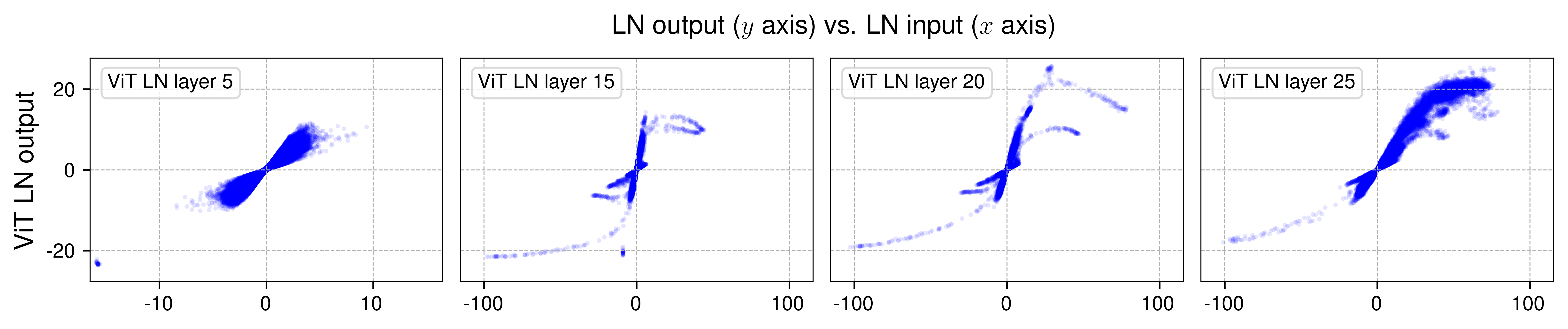
Figure 2 (Zhu et al., 2025): LN output vs. LN input for four layers of ViT-B. Earlier layers (left) show a roughly linear mapping; deeper layers (right) develop a pronounced tanh-shaped S-curve. Each point is one (token, channel) pair sampled from a mini-batch. The progressive saturation of the envelope motivates replacing LN with a learned tanh.
2.2 Deriving the Envelope
We now derive why many linear functions with varying slopes collectively produce an S-shaped curve. For clarity, work in the RMSNorm setting (zero mean) with a single channel, so \(\mu_t = 0\) and \(\gamma = 1\):
\[y = \frac{x}{\sigma_t}\]
Let \(\sigma_t \sim p(\sigma)\) for some distribution on \(\mathbb{R}_{>0}\). Treating \(x\) as a fixed input and averaging over tokens:
\[\mathbb{E}_\sigma[y \mid x] = x \cdot \mathbb{E}\!\left[\frac{1}{\sigma}\right]\]
This is linear in \(x\) for any finite \(\mathbb{E}[1/\sigma]\) — consistent with the near-linear behavior at the origin.
For large \(|x|\), however, \(x/\sigma\) is large only when \(\sigma\) is small. If \(p(\sigma)\) has a lower bound \(\sigma_{\min} > 0\), then \(y \leq |x|/\sigma_{\min}\), but the conditional distribution of \(\sigma\) given that \(|x|/\sigma\) is large concentrates on small \(\sigma\). The average output saturates relative to \(|x|\) as the weight shifts to the small-\(\sigma\) (steep-slope) tokens.
As a concrete case: suppose \(\sigma \sim \text{Uniform}[a, b]\) with \(0 < a < b\). Then:
\[\mathbb{E}\!\left[\frac{x}{\sigma}\right] = x \cdot \frac{1}{b-a}\ln\!\frac{b}{a}\]
which is linear. For the envelope (the maximum achievable output for a given \(x\) over the family of lines), define \(F(x) = \sup_{\sigma \in [a,b]} x/\sigma\). For \(x > 0\), \(F(x) = x/a\), which is linear. But the average output, considered as a function of where the data point \((x, y)\) falls relative to the cloud of all token points, traces an S-shape because the density of points at extreme \(y\) values is lower — large \(|y|\) requires small \(\sigma\), which is a low-probability event.
More precisely: the conditional mean \(\mathbb{E}[y \mid x]\) is linear, but the marginal distribution of \((x, y)\) pairs over all tokens is S-shaped because \(x\) and \(\sigma\) are correlated in a trained network — tokens with large activation magnitude also tend to have large \(\sigma\), so their output is compressed back toward the mean.
In a trained network, the LayerNorm input \(x\) is itself the output of an attention or FFN sublayer. The scale of \(x\) is not independent of \(\sigma\): tokens with larger norm tend to have larger \(\sigma\). This correlation is precisely what creates the saturation — large \(|x|\) tokens have large \(\sigma\), so \(x/\sigma\) does not grow proportionally with \(|x|\).
This exercise establishes the key geometric observation underlying the tanh analogy — that a family of lines with varying slopes, centered near the origin, collectively traces an S-shaped curve.
Prerequisites: 2.2 Deriving the Envelope
Let \(f_\sigma(x) = x/\sigma\) for \(\sigma\) drawn i.i.d. from a distribution \(p(\sigma)\) on \(\mathbb{R}_{>0}\) with finite \(\mathbb{E}[1/\sigma]\) and \(\mathbb{E}[1/\sigma^2]\). Define the aggregate mapping \(g(x) = \mathbb{E}_\sigma[f_\sigma(x)] = x \cdot \mathbb{E}[1/\sigma]\).
Show that \(g(x)\) is linear in \(x\), hence not S-shaped on its own.
Now suppose instead that we observe the mapping at a fixed output scale: we plot points \((x, y)\) where \(y = x/\sigma\) and \(\sigma\) is sampled independently of \(x\), but \(x\) itself has some distribution \(q(x)\). Show that if \(\sigma\) and \(|x|\) are positively correlated (tokens with large \(|x|\) tend to have large \(\sigma\)), the marginal cloud of \((x, y)\) pairs has compressed extremes — i.e., the curve \(x \mapsto \mathbb{E}[y \mid x]\) is sublinear for large \(|x|\) and superlinear for small \(|x|\), giving an S-shape.
As a concrete case: let \(\sigma = c|x| + \epsilon\) for constants \(c > 0\), \(\epsilon > 0\) (a crude model of the correlation). Compute \(\mathbb{E}[y \mid x]\) and show it saturates as \(|x| \to \infty\).
Key insight: Linear functions \(y = x/\sigma\) are individually linear, but correlation between \(\sigma\) and \(|x|\) in trained networks compresses the aggregate mapping at large \(|x|\), creating the S-shape.
Sketch:
(a) \(g(x) = \mathbb{E}_\sigma[x/\sigma] = x \mathbb{E}[1/\sigma]\). Since \(\mathbb{E}[1/\sigma]\) is a finite constant independent of \(x\), \(g\) is linear. No S-shape arises from averaging over \(\sigma\) alone.
(b) If \(\sigma\) and \(|x|\) are positively correlated, then conditioning on large \(|x|\) shifts the distribution of \(\sigma\) toward larger values. Therefore \(\mathbb{E}[\sigma \mid x] > \mathbb{E}[\sigma]\) when \(|x|\) is large, and \(\mathbb{E}[y \mid x] = x \cdot \mathbb{E}[1/\sigma \mid x] < x \cdot \mathbb{E}[1/\sigma]\). The effective slope \(\mathbb{E}[1/\sigma \mid x]\) decreases as \(|x|\) increases, producing a concave (sub-linear) envelope for \(x > 0\) — and by symmetry, a convex (super-linear then saturating) envelope for \(x < 0\). Together these give an S-shape.
(c) With \(\sigma = c|x| + \epsilon\): \[\mathbb{E}[y \mid x] = \frac{x}{c|x| + \epsilon} = \frac{\text{sgn}(x)}{c + \epsilon/|x|}\] As \(|x| \to \infty\): \(\mathbb{E}[y \mid x] \to \text{sgn}(x)/c\). The output saturates at \(\pm 1/c\), independent of \(|x|\). Near \(x = 0\): \(\mathbb{E}[y \mid x] \approx x/\epsilon\), which is linear. This is precisely the qualitative shape of tanh.
3. Dynamic Tanh (DyT) ⚡
3.1 Formal Definition
Definition (Dynamic Tanh). Dynamic Tanh (DyT) is defined as:
\[\text{DyT}(x) = \gamma \odot \tanh(\alpha x) + \beta\]
where: - \(\alpha \in \mathbb{R}\) is a single learnable scalar shared across all channels, - \(\gamma, \beta \in \mathbb{R}^d\) are learnable per-channel affine parameters (matching the role of \(\gamma, \beta\) in LayerNorm), - Default initialization: \(\alpha_0 = 0.5\), \(\gamma = \mathbf{1}\), \(\beta = \mathbf{0}\).
DyT is a drop-in replacement: it occupies exactly the same position as LayerNorm or RMSNorm in the Transformer block (Pre-Norm position, applied before the attention or FFN sublayer). No other architectural changes are required.
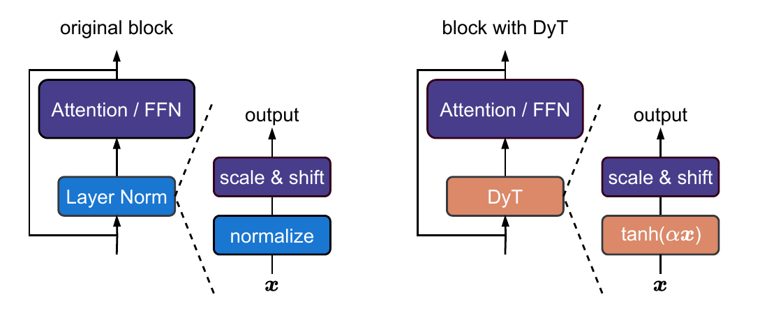
Figure 1 (Zhu et al., 2025): The DyT substitution. Left: a standard Pre-Norm Transformer block with a LayerNorm (normalize → scale & shift). Right: the DyT block, where the normalize step is replaced by \(\tanh(\alpha x)\); the scale & shift affine parameters \(\gamma, \beta\) are retained. No other changes to the architecture are needed.
The tanh function satisfies \(\tanh(x) = (e^x - e^{-x})/(e^x + e^{-x})\) and maps \(\mathbb{R} \to (-1, 1)\). The scalar \(\alpha\) controls the slope at the origin: \(\tanh'(0) = 1\), so \((\tanh \circ \alpha \cdot)(0)' = \alpha\).
Fixing \(\alpha = 1\) and applying \(\tanh\) directly would impose a fixed scale on all layers. But deeper layers have larger input variance (since residual connections accumulate signal across many layers), and these layers need a softer saturation curve — achieved by smaller \(\alpha\). The scalar \(\alpha\) effectively adapts the operating range of tanh to the layer’s input statistics without requiring explicit computation of per-token statistics.
3.2 The Role of Alpha
Empirically, \(\alpha\) converges during training to track the inverse standard deviation of the layer’s input activations:
\[\alpha \approx \frac{1}{\text{std}(x)}\]
This is not a coincidence — in the linear regime of tanh (\(|\alpha x_i| \ll 1\)), \(\tanh(\alpha x_i) \approx \alpha x_i\), so \(\text{DyT}(x) \approx \alpha \gamma \odot x + \beta\), which matches RMSNorm’s output \(\gamma \odot x / \text{RMS}(x)\) when \(\alpha \approx 1/\text{RMS}(x)\).
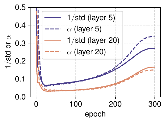
Figure 5a (Zhu et al., 2025): Evolution of \(\alpha\) (dashed) and \(1/\text{std}\) (solid) over 300 training epochs for two DyT layers in ViT-B. Both quantities decrease sharply in early training and then rise together, confirming that \(\alpha\) tracks the inverse standard deviation of layer inputs throughout optimization.
Ablation results on ViT-B (ImageNet top-1):
| Configuration | Accuracy |
|---|---|
| DyT with learned \(\alpha\) | 82.5% |
| Fixed \(\alpha = 1\) | 81.1% |
| No \(\alpha\) (pure tanh + affine) | 81.1% |
The \(\alpha\) scalar is responsible for roughly 1.4 percentage points of the performance gap, confirming it functions as a learned normalization scale.
After training, \(\alpha\) values are larger in deeper layers — consistent with deeper layers having larger input standard deviations (due to residual accumulation), and needing smaller effective scale \(1/\alpha\) to keep \(\alpha x\) in the linear regime of tanh.
3.3 Initialization Sensitivity in LLMs
For large language models, \(\alpha_0 = 0.5\) (used for ViT) is inadequate. Wider models have larger weight matrices, producing larger pre-activation magnitudes, requiring smaller \(\alpha\) to keep \(\alpha x\) near zero at initialization (where tanh is approximately linear and the network is in a “lazy” training regime).
Empirically determined \(\alpha_0\) for LLaMA:
| Model | Attention DyT | Other DyT |
|---|---|---|
| LLaMA-7B | 0.8 | 0.2 |
| LLaMA-70B | 0.2 | 0.05 |
This width-dependence of \(\alpha_0\) is a practical complication absent in vision models. It implies that out-of-the-box DyT requires tuning \(\alpha_0\) as a function of model width — partially undermining the simplicity motivation.
3.4 Experimental Results
DyT matches or exceeds LN/RMSNorm across all modalities:
| Task | Model | LN/RMSNorm | DyT | \(\Delta\) |
|---|---|---|---|---|
| Vision | ViT-L/ImageNet top-1 | 83.1% | 83.6% | +0.5% |
| Generative | DiT-B/ImageNet FID | 64.9 | 63.9 | −1.0 |
| Language | LLaMA-7B avg. zero-shot | 0.513 | 0.513 | 0 |
| Speech | wav2vec-2.0-L val loss | 1.92 | 1.91 | −0.01 |
Efficiency (LLaMA-7B, BF16): 42% reduction in per-layer training time; 8.2% full-model training speedup. The gain comes from eliminating the per-token mean/variance computation and associated synchronization.
3.5 Ablation on the Squashing Function
The choice of tanh is not arbitrary. The following saturating functions were evaluated on ViT-B:
| Function | ViT-B Top-1 |
|---|---|
| Identity (no squash) | diverged |
| Sigmoid | 81.6% |
| Hardtanh | 82.2% |
| Tanh | 82.5% |
Tanh wins due to two properties: smoothness (unlike Hardtanh, which has zero gradient in the saturated region) and zero-centeredness (unlike sigmoid, which outputs in \((0, 1)\) rather than \((-1, 1)\)). The identity function diverges because without any squashing, there is no mechanism to prevent signal explosion across layers.
This exercise formalizes the empirical observation that \(\alpha\) converges to \(1/\text{std}(x)\) by framing it as a least-squares problem.
Prerequisites: 3.2 The Role of Alpha
Fix a layer with input \(x \in \mathbb{R}^d\) drawn from a zero-mean distribution with standard deviation \(\sigma > 0\) per coordinate (i.e., the RMSNorm setting). Set \(\gamma = \mathbf{1}\), \(\beta = \mathbf{0}\) for simplicity.
Define the target output as \(\text{RMSNorm}(x) = x/\sigma\) and the DyT output as \(\text{DyT}(x; \alpha) = \tanh(\alpha x)\) (elementwise). Minimize the mean squared error over the input distribution:
\[\hat{\alpha} = \arg\min_{\alpha \geq 0} \mathbb{E}_x\!\left[\|\tanh(\alpha x) - x/\sigma\|^2\right]\]
In the regime where \(|\alpha x_i| \ll 1\) for all \(i\) (most activations in the linear part of tanh), show that the optimal \(\alpha\) is approximately \(1/\sigma\).
Explain qualitatively why the true optimum (without the small-argument approximation) satisfies \(\hat{\alpha} < 1/\sigma\), and why this systematic underestimate is harmless.
Key insight: In the linear regime of tanh, DyT is approximately \(\text{id} \cdot \alpha\), and minimizing MSE to \(x/\sigma\) directly gives \(\alpha = 1/\sigma\). The underestimate in the nonlinear regime is harmless because the residual error is a second-order correction.
Sketch:
(a) For \(|\alpha x_i| \ll 1\), use \(\tanh(u) \approx u - u^3/3\). To first order: \(\tanh(\alpha x_i) \approx \alpha x_i\). The MSE becomes: \[\mathbb{E}\!\left[(\alpha x_i - x_i/\sigma)^2\right] = (\alpha - 1/\sigma)^2 \mathbb{E}[x_i^2] = (\alpha - 1/\sigma)^2 \sigma^2\] Minimizing over \(\alpha\) gives \(\hat{\alpha} = 1/\sigma\).
(b) For the full nonlinear tanh: \(\tanh(\alpha x_i) \leq \alpha x_i\) for \(x_i > 0\) (tanh is concave on \(\mathbb{R}_{>0}\)), so the tanh output is systematically smaller than \(\alpha x_i\) in magnitude. To compensate, the optimizer nudges \(\alpha\) slightly above \(1/\sigma\) — but simultaneously, for large-magnitude tokens (which tanh saturates), increasing \(\alpha\) beyond \(1/\sigma\) increases saturation error. The optimum balances these forces and lies near \(1/\sigma\). The deviation is \(O(\alpha^3 \mathbb{E}[x^4]/\sigma^2)\), a fourth-moment correction that is small when activations are approximately Gaussian.
4. Toward a Theory: Four Properties 📐
The DyT paper demonstrates that tanh works as a normalization replacement. The Derf paper asks the deeper question: why tanh? Are there better alternatives? To answer this, the authors identify four properties that any pointwise normalization replacement must satisfy for training to succeed.
Let \(f: \mathbb{R} \to \mathbb{R}\) be the core scalar function (before the affine wrap). The framework instantiates any candidate as \(F(x) = \gamma \odot f(\alpha x + s) + \beta\) and evaluates on ViT-B ImageNet and DiT-B FID.
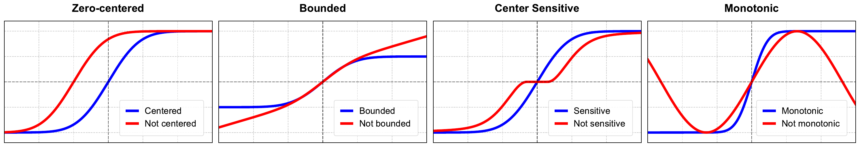
Figure 1 (Chen et al., 2025): Visual illustration of the four properties. In each panel, the blue curve satisfies the property and the red curve violates it. Left to right: (1) Zero-centeredness — centered vs. horizontally shifted; (2) Boundedness — bounded vs. unbounded growth; (3) Center sensitivity — steep vs. flat slope at the origin; (4) Monotonicity — monotone vs. non-monotone (hump-shaped). Any valid normalization replacement must match the blue profile in all four panels.
4.1 Property 1: Zero-Centeredness
Property 1 (Zero-Centeredness). The function \(f\) must satisfy \(f(0) \approx 0\) and be balanced (odd or approximately odd) around the origin. Formally: horizontally shifting \(f\) by \(\lambda\) (i.e., using \(f(x + \lambda)\)) or vertically shifting by \(\lambda\) (i.e., \(f(x) + \lambda\)) should incur negligible accuracy loss for small \(|\lambda|\), but shifts of \(|\lambda| \geq 2\) degrade performance measurably.
Rationale: If \(f\) is offset from zero, the residual connection in the Transformer block \(x \leftarrow x + \text{Sublayer}(F(x))\) receives a biased input. Over many layers, a constant offset accumulates into a systematic drift in activation statistics, analogous to the covariate shift that normalization was designed to prevent. Zero-centering keeps the activations in the gradient-rich regime of subsequent nonlinearities.
4.2 Property 2: Boundedness
Property 2 (Boundedness). There exist finite constants \(a < b\) such that \(a \leq f(x) \leq b\) for all \(x \in \mathbb{R}\).
Rationale: Without bounded output, large-magnitude inputs pass through DyT/Derf with magnitude proportional to \(|x|\) (or worse), and residual connections accumulate these unbounded activations across depth. In experiments, replacing tanh with unbounded functions (linear, logsign \(= x/|x| \cdot \log(1+|x|)\), arcsinh) leads to divergence. Clipping these unbounded functions to a finite range \([-C, C]\) recovers performance, confirming that boundedness per se — not the specific saturating shape — is the critical structural requirement.
The function \(f(x) = \text{arcsinh}(x) = \ln(x + \sqrt{x^2+1})\) is unbounded. Applied as DyT with arcsinh, ViT-B training diverges. Clipping to \([-3, 3]\): training succeeds and achieves competitive accuracy. The clipping imposes boundedness artificially, confirming Property 2.
4.3 Property 3: Center Sensitivity
Property 3 (Center Sensitivity). The function \(f\) must have nonzero (and preferably large) derivative at \(x = 0\). Formally: if \(f\) has a flat “dead zone” around \(x = 0\) of width \(\lambda\) (i.e., \(f'(x) = 0\) for \(|x| \leq \lambda/2\)), then: - \(\lambda \leq 1.0\): no significant performance degradation - \(\lambda \geq 1.0\): accuracy begins dropping - \(\lambda \geq 3.0\): training diverges
Rationale: The bulk of activations in a trained network concentrate near zero (approximately Gaussian with small variance). If the function is flat near zero, gradients vanish for the majority of tokens — this is the deep-learning analogue of the dying ReLU problem. A steep slope at the origin ensures strong gradient signal for the most common activation magnitudes.
4.4 Property 4: Monotonicity
Property 4 (Monotonicity). The function \(f\) must be non-decreasing (or non-increasing) everywhere on \(\mathbb{R}\).
Rationale: Non-monotone functions (hump-shaped, oscillatory, or with local extrema) create regions where the gradient of the loss w.r.t. the pre-activation has opposite sign for inputs on opposite sides of a local maximum. This sign conflict means weight updates that improve performance for some tokens actively harm others. Empirically:
| Function type | ViT-B accuracy |
|---|---|
| Monotone (tanh family) | 82.3%–82.6% |
| Non-monotone variants | 80.7%–81.6% |
The gap is consistent across many non-monotone candidates, confirming monotonicity as a reliable property rather than a coincidence of one bad candidate.
Remark. The four properties jointly define a manageable search space: S-shaped, zero-centered, bounded, smooth, monotone scalar functions. This is precisely the family of sigmoid-like or tanh-like functions, vindicating the original DyT design choice on principled grounds.
This exercise grounds the four abstract properties in concrete functions, verifying that the framework correctly classifies tanh as valid and ReLU/linear as invalid.
Prerequisites: 4. Toward a Theory: Four Properties
Verify that \(f(x) = \tanh(x)\) satisfies all four properties (zero-centeredness, boundedness, center sensitivity, monotonicity). Provide a one-sentence justification for each.
Show that \(f(x) = \text{ReLU}(x) = \max(0, x)\) fails exactly one of the four properties. Identify which one and explain why this makes ReLU an invalid normalization replacement.
Show that \(f(x) = x\) (identity/linear) fails exactly one of the four properties. Identify which one.
Conclude by explaining why the theory predicts that neither ReLU nor linear can serve as normalization replacements, and check that this prediction matches the empirical divergence results.
Key insight: tanh is the canonical function satisfying all four properties. ReLU fails center sensitivity (flat for \(x < 0\)); linear fails boundedness. Both failures are fatal to training stability.
Sketch:
(a) tanh satisfies all four: - Zero-centered: \(\tanh(0) = 0\) and \(\tanh\) is an odd function. - Bounded: \(-1 < \tanh(x) < 1\) for all \(x\). - Center sensitive: \(\tanh'(0) = 1 > 0\), so there is no dead zone at the origin. - Monotone: \(\tanh'(x) = \text{sech}^2(x) > 0\) for all \(x\).
(b) ReLU fails Property 3 (center sensitivity): \(\text{ReLU}'(x) = 0\) for \(x < 0\), creating a dead zone of effective width \(\lambda = \infty\) on the negative half-line. The majority of tokens with negative activations receive zero gradient through the normalization replacement, causing gradient starvation. ReLU does satisfy zero-centering (approximately, since \(\text{ReLU}(0) = 0\)), boundedness-from-below (output \(\geq 0\); fails boundedness-from-above — so actually fails two properties), and monotonicity.
(c) Linear fails Property 2 (boundedness): \(f(x) = x\) is unbounded above and below. Large-magnitude inputs pass through unattenuated, causing activation explosion via residual connections across depth.
(d) The theory predicts divergence for both ReLU (dead zone → gradient starvation) and linear (unbounded → explosion). This matches the empirical ablation: identity/linear diverges, and one-sided functions (sigmoid, which has a dead zone for large negative inputs relative to its center) underperform. The theory thus has correct qualitative predictions for all tested functions.
5. Dynamic erf (Derf) 🎯
5.1 Formal Definition
Definition (Dynamic erf). Derf is defined as:
\[\text{Derf}(x) = \gamma \odot \text{erf}(\alpha x + s) + \beta\]
where: - \(\text{erf}(x) = \frac{2}{\sqrt{\pi}} \int_0^x e^{-t^2}\, dt\) is the error function (related to the Gaussian CDF by \(\Phi(x) = \frac{1}{2}[1 + \text{erf}(x/\sqrt{2})]\)) - \(\alpha \in \mathbb{R}\) is a learnable scalar controlling input scale (same role as in DyT) - \(s \in \mathbb{R}\) is a learnable scalar shift — an extra degree of freedom absent in DyT - \(\gamma, \beta \in \mathbb{R}^d\) are learnable per-channel affine parameters - Default initialization: \(\alpha_0 = 0.5\), \(s_0 = 0\), \(\gamma = \mathbf{1}\), \(\beta = \mathbf{0}\)
At initialization with \(s_0 = 0\), Derf reduces to \(\gamma \odot \text{erf}(\alpha x) + \beta\), which is symmetric (odd) and zero-centered. The shift \(s\) allows the operating center to migrate during training if needed.
The error function satisfies \(\text{erf}(-x) = -\text{erf}(x)\) (odd), \(\text{erf}(0) = 0\) (zero-centered), \(|\text{erf}(x)| < 1\) (bounded), \(\text{erf}'(x) = \frac{2}{\sqrt{\pi}} e^{-x^2} > 0\) (monotone). All four properties of Section 4 are satisfied.
5.2 Function Search Procedure
To justify choosing erf over the many other functions satisfying the four properties, the authors performed a systematic search over candidate scalar functions. The search space included:
- Function families: polynomial, rational, exponential, logarithmic, trigonometric, and CDF-based (Gaussian, Laplace, Cauchy, logistic)
- Transformations: translation, scaling, mirroring, rotation, clipping
- Instantiation: each candidate \(h\) was wrapped as \(F(x) = \gamma \odot h(\alpha x + s) + \beta\) and evaluated with \(\alpha_0 = 0.5\), \(s_0 = 0\), \(\gamma = \mathbf{1}\), \(\beta = \mathbf{0}\)
Over 20 candidate functions were evaluated on ViT-Base ImageNet top-1 accuracy and DiT-B FID at a fixed compute budget. erf ranked first on both metrics.
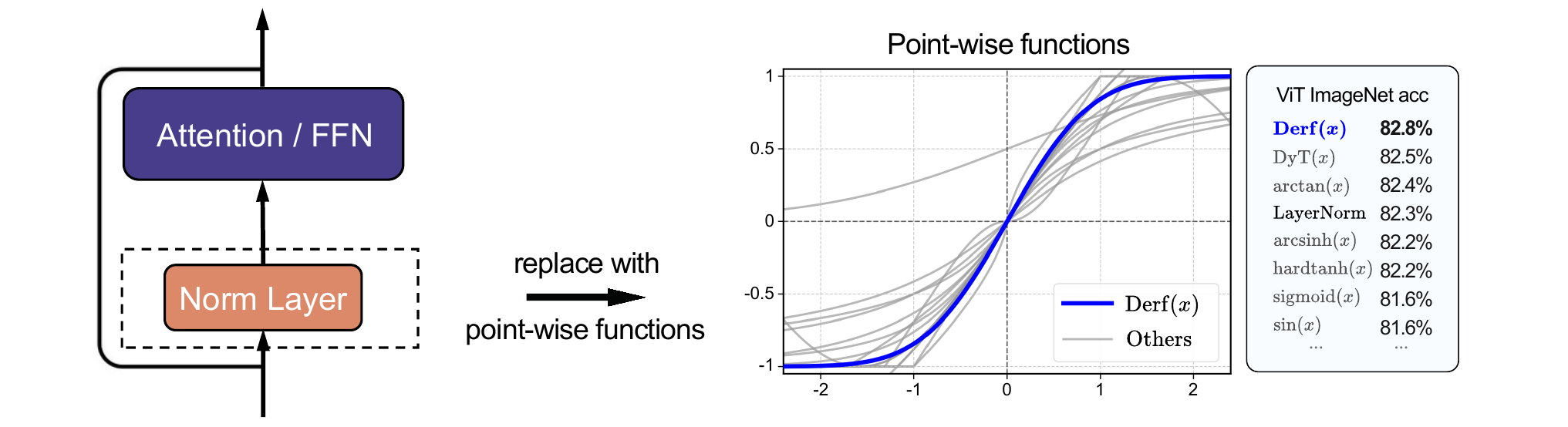
Figure (Chen et al., 2025): Summary of the function search. The center plot shows the shape of all candidate point-wise functions; \(\text{erf}(x)\) (Derf, blue) saturates faster near the origin than \(\tanh(x)\) (DyT) and much faster than \(\arctan(x)\). The ranking table on the right shows ViT-B ImageNet top-1 accuracy for each candidate — erf/Derf tops the list at 82.8%, outperforming DyT (82.5%) and LayerNorm (82.3%).
5.3 Why erf Beats tanh
Three reasons:
1. Higher derivative at the origin. \(\text{erf}'(0) = 2/\sqrt{\pi} \approx 0.798\), while the effective derivative at zero for \(\tanh\) (before the \(\alpha\) scaling) is \(\tanh'(0) = 1\). However, after accounting for the \(\alpha\) scaling in both functions, what matters is the shape of the derivative near zero. erf has a Gaussian derivative \(\text{erf}'(x) = \frac{2}{\sqrt{\pi}} e^{-x^2}\) which falls off more slowly than \(\tanh'(x) = \text{sech}^2(x)\) for small \(|x|\) — erf maintains higher center sensitivity over a wider activation range.
2. Better gradient characteristics. The Gaussian derivative \(e^{-x^2}\) has heavier tails than \(\text{sech}^2(x)\) for moderate \(|x|\) (say \(|x| \in [1, 3]\)), meaning erf provides stronger gradient signal for slightly off-center activations.
3. erf \(\neq\) scaled tanh. The approximation \(\text{erf}(x) \approx \tanh(\sqrt{\pi}/2 \cdot x)\) is widely cited. The Derf paper explicitly tests scaled tanh (i.e., \(\tanh(\sqrt{\pi}/2 \cdot \alpha x)\)) and finds it performs strictly worse than true erf. The approximation error is measurable and performance-relevant — erf and scaled tanh are not interchangeable in practice.
5.4 Experimental Results
Derf consistently outperforms both LayerNorm and DyT:
| Task | Model | LayerNorm | DyT | Derf | \(\Delta\) vs LN |
|---|---|---|---|---|---|
| Vision | ViT-B ImageNet top-1 | 82.3% | 82.5% | 82.8% | +0.5% |
| Vision | ViT-L ImageNet top-1 | 83.1% | 83.6% | 83.8% | +0.7% |
| Generative | DiT-B FID | 64.93 | 63.71 | 63.23 | −1.70 |
| Generative | DiT-L FID | 45.91 | 45.66 | 43.94 | −1.97 |
| Speech | wav2vec-L val loss | 1.92 | 1.91 | 1.90 | −0.02 |
| DNA | HyenaDNA accuracy | 85.2% | 85.2% | 85.7% | +0.5% |
| Language | GPT-2 val loss | 2.94 | 2.97 | 2.94 | 0 |
On generative modeling (DiT), the gains over LayerNorm are particularly striking: −1.97 FID on DiT-L, a substantial improvement in sample quality. On language modeling (GPT-2), Derf matches LayerNorm — DyT slightly underperforms — suggesting the language modeling objective is less sensitive to the normalization mechanism.
On ViT-B, Derf achieves higher training loss (0.2681) than LayerNorm (0.2623) yet better validation accuracy (82.8% vs. 82.3%). This pattern — worse train loss, better generalization — is consistent across DyT and Derf and points to an implicit regularization story explored in Section 6.
This exercise uses the train/validation loss discrepancy to reason about the implicit regularization role of LayerNorm.
Prerequisites: 5.4 Experimental Results, 6.1 Implicit Regularization by Normalization
The Derf paper reports the following on ViT-B:
| Method | Training loss | Top-1 accuracy |
|---|---|---|
| LayerNorm | 0.2623 | 82.3% |
| Derf | 0.2681 | 82.8% |
Assuming no confounds (same architecture, same optimizer, same data), what does higher training loss combined with higher validation accuracy imply about the generalization gap? Is Derf underfitting, overfitting, or neither relative to LayerNorm?
Formalize the claim that LayerNorm acts as an implicit regularizer. Specifically: what constraint does LayerNorm impose on the feature distribution at each layer, and how is this analogous to \(L^2\) regularization?
Under this regularization interpretation, why might removing the normalization constraint allow the model to fit the training set less tightly yet generalize better — i.e., what is the mechanism by which a weaker inductive bias could improve generalization?
Key insight: LayerNorm imposes a per-layer unit-variance constraint that acts as implicit regularization. This constraint reduces effective model capacity and can prevent overfitting — but it can also prevent the model from learning the optimal feature scale, so removing it can improve generalization when the constraint is miscalibrated.
Sketch:
(a) Higher training loss + higher validation accuracy means Derf has a smaller generalization gap (validation - training loss gap) than LayerNorm, not that it is underfitting. LayerNorm achieves lower training loss (fits the training data better) but higher validation loss (generalizes worse). Derf is closer to the optimal bias-variance tradeoff for this task.
(b) LayerNorm forces \(\text{Var}[x_i] = 1\) (and \(\mathbb{E}[x_i] = 0\)) at each layer — a hard constraint on the feature distribution. This is analogous to \(L^2\) regularization in the following sense: \(L^2\) regularization penalizes large weight norms, restricting the set of reachable functions. LayerNorm restricts the set of reachable activation distributions — only functions whose intermediate activations have unit variance are in the effective hypothesis class. This is a structural constraint that reduces the Rademacher complexity of the model.
(c) The implicit regularization from LayerNorm is not data-adaptive — it enforces unit variance regardless of whether that is the right scale for the task. For ImageNet classification, the optimal feature scales at various layers may deviate from unit variance. Derf allows the network to learn task-aligned feature scales (via \(\alpha\), \(\gamma\)), which can find a better solution in hypothesis space. The better generalization is a consequence of having the right bias (pointwise boundedness via tanh/erf) without the wrong bias (forced unit variance). This is consistent with the bias-variance tradeoff: removing LayerNorm’s hard constraint reduces bias (lower restriction on function class) in a beneficial direction.
6. Why Do Pointwise Functions Work At All? 💡
Surprisingly, removing normalization from Transformers — a component long considered essential for training stability — not only does not hurt performance, it consistently improves it. Two complementary mechanisms explain this.
6.1 Implicit Regularization by Normalization
LayerNorm and RMSNorm impose per-token, per-layer constraints on activation statistics. This is a form of implicit regularization: the model’s effective hypothesis class is restricted to functions whose intermediate representations have unit variance (and zero mean, in the LayerNorm case).
This constraint is not learned from data — it is architecturally imposed regardless of the task. For many vision and speech tasks, the optimal activation scale at each layer is not exactly unit variance, and forcing it there prevents the model from finding its preferred operating point. DyT and Derf replace this hard constraint with a soft learned squashing: the network can adjust \(\alpha\) and \(\gamma\) to set the effective scale at each layer, allowing a task-specific operating regime.
The empirical signature of this mechanism is the train-loss / val-accuracy inversion: LayerNorm achieves lower training loss (it can, in principle, fit training data at unit variance) but higher validation loss — the unit-variance constraint was miscalibrated for generalization.
6.2 Statistics-Free Computation
LayerNorm and RMSNorm compute statistics (\(\mu_t\), \(\sigma_t\)) from the current token’s activations. This computation is deterministic given the token, but it introduces a subtle cross-token dependency in the normalization output: two tokens with the same value \(x_i\) at channel \(i\) receive different normalized outputs if their overall feature vectors have different means/variances. The normalization is thus context-sensitive — the output for token \(t\) at channel \(i\) depends on the values at all other channels of the same token.
DyT and Derf are statistics-free: the function \(\text{DyT}(x_i) = \gamma_i \tanh(\alpha x_i) + \beta_i\) depends only on \(x_i\), not on any other channel. This makes the normalization replacement a pure elementwise transformation with no cross-channel interaction.
In Transformer architectures, cross-channel interaction is the job of the weight matrices in attention (\(W_Q, W_K, W_V, W_O\)) and the FFN (\(W_1, W_2\)). Having normalization also mix channels (via \(\sigma\), which depends on all channels) creates a redundant and potentially conflicting source of cross-channel computation. Removing it lets the learned weight matrices govern all cross-channel interactions cleanly.
DyT and Derf explicitly fail to replace BatchNorm in classical ConvNets. On ResNet-50, replacing BatchNorm with DyT drops top-1 accuracy from 76.2% to 68.9% — a catastrophic degradation. The likely reason: BatchNorm appears after every weight layer in a ResNet (dense application), while LayerNorm appears sparsely at the start of sublayers in a Pre-Norm Transformer. Dense application of a pointwise squashing function without explicit normalization leaves no mechanism to prevent activation drift across the many weight layers of a ResNet. The success of DyT/Derf is specific to the Pre-Norm Transformer architecture.
7. Limitations ⚠️
BatchNorm incompatibility. DyT and Derf cannot replace BatchNorm. ResNet-50 accuracy drops from 76.2% to 68.9% (DyT). The hypothesis: BatchNorm is applied densely (after every weight layer), and its primary role in ConvNets is covariate shift correction across batch statistics — a function that a pointwise squasher cannot replicate. The sparse placement of LayerNorm in Transformers (once per sublayer, in Pre-Norm position) means the normalization role is less critical per-occurrence, making pointwise substitution viable.
LLM initialization sensitivity. For large language models, the default \(\alpha_0 = 0.5\) fails; correct initialization must scale inversely with model width. LLaMA-7B requires \(\alpha_0 \in \{0.2, 0.8\}\) depending on sublayer type; LLaMA-70B requires \(\{0.05, 0.2\}\). This re-introduces a width-dependent hyperparameter that practitioners must tune — partially negating the simplicity advantage over LayerNorm. The sensitivity is more pronounced for DyT than for Derf (which has the additional shift \(s\) to absorb initialization error), but both require care.
Scope limited to Pre-Norm Transformers. All experiments use Pre-Norm architectures (where normalization precedes the sublayer computation). Post-Norm Transformers (where normalization follows the sublayer, as in the original “Attention Is All You Need”) are known to be harder to train, with or without normalization. Whether DyT/Derf can replace normalization in Post-Norm settings — or in hybrid architectures like DeepNorm — is unstudied.
Theoretical gap. The four-property framework (Section 4) identifies necessary conditions empirically, but there is no formal proof that these conditions are sufficient, nor any PAC-style generalization bound that explains why removing per-token normalization improves validation performance. The train-loss / val-accuracy inversion (Section 6) is interpreted heuristically; a formal characterization of the implicit regularization mechanism remains open.
References
| Reference Name | Brief Summary | Link to Reference |
|---|---|---|
| Transformers without Normalization | Introduces DyT \(= \gamma \odot \tanh(\alpha x) + \beta\) as a drop-in LayerNorm replacement; empirically shows LN output \(\approx\) tanh of LN input in trained models; reports 8.2% LLaMA-7B training speedup | https://arxiv.org/abs/2503.10622 |
| Stronger Normalization-Free Transformers | Formalizes four necessary properties for pointwise norm replacements; introduces Derf \(= \gamma \cdot \text{erf}(\alpha x + s) + \beta\) via systematic function search; outperforms DyT and LN across vision, generative, speech, DNA, language tasks | https://arxiv.org/abs/2512.10938 |
| Layer Normalization | Original LayerNorm paper; normalizes across the feature dimension per token; foundational for Transformer training stability | https://arxiv.org/abs/1607.06450 |
| Root Mean Square Layer Normalization | RMSNorm — drops mean centering, normalizes by RMS only; faster than LayerNorm with equivalent or better training stability; used in LLaMA and most modern LLMs | https://arxiv.org/abs/1910.07467 |