🔥 torch.compile: Full-Stack Survey
Table of Contents
- 1. Motivation and Architecture at a Glance
- 2. TorchDynamo: Python Bytecode Interception
- 3. The FX Intermediate Representation
- 4. AOTAutograd: Ahead-of-Time Joint Tracing
- 5. PrimTorch: Operator Decomposition
- 6. TorchInductor: Loop-Level IR and Kernel Generation
- 7. End-to-End Data Flow
- 8. Guards and Recompilation in Depth
- 9. torch.compile Usage Modes
- References
1. Motivation and Architecture at a Glance
PyTorch’s eager execution model is maximally flexible: every operator call dispatches immediately through the C10 Dispatcher, the Autograd Engine records a tape node, and the kernel launches on the device. The interpreter overhead incurred by Python and the inability to observe more than one operator at a time preclude two major classes of optimization:
- Kernel fusion — adjacent elementwise or reduction operations can be merged into a single kernel, eliminating redundant HBM round-trips.
- Cross-pass optimization — the backward graph is unknown at forward time, so decisions such as which activations to save (rather than recompute) cannot be made globally.
torch.compile layers a multi-stage compilation pipeline in front of eager execution without abandoning Python’s dynamism. The four stages are:
| Stage | Input | Output | Principal invariant |
|---|---|---|---|
| TorchDynamo | Python bytecode frames | FX graph fragments + guards | Semantically equivalent to eager; guards certify validity |
| AOTAutograd | FX forward graph | Paired forward + backward FX graphs | Joint functional graph; all mutations and aliases resolved |
| PrimTorch | ATen-level FX graph | Prim-level FX graph (~250 ops) | Closed, stable operator surface any backend can implement |
| TorchInductor | Prim-level FX graph | Triton / C++/OpenMP source | Optimal loop structure; fused kernels; hardware-specific |
Performance headline: Ansel et al. (ASPLOS 2024) report a geometric mean of 2.27× inference and 1.41× training speedup over eager execution on an NVIDIA A100 across 180+ real-world models, while achieving a 99% graph capture rate — compared to approximately 50% for the earlier TorchScript approach.
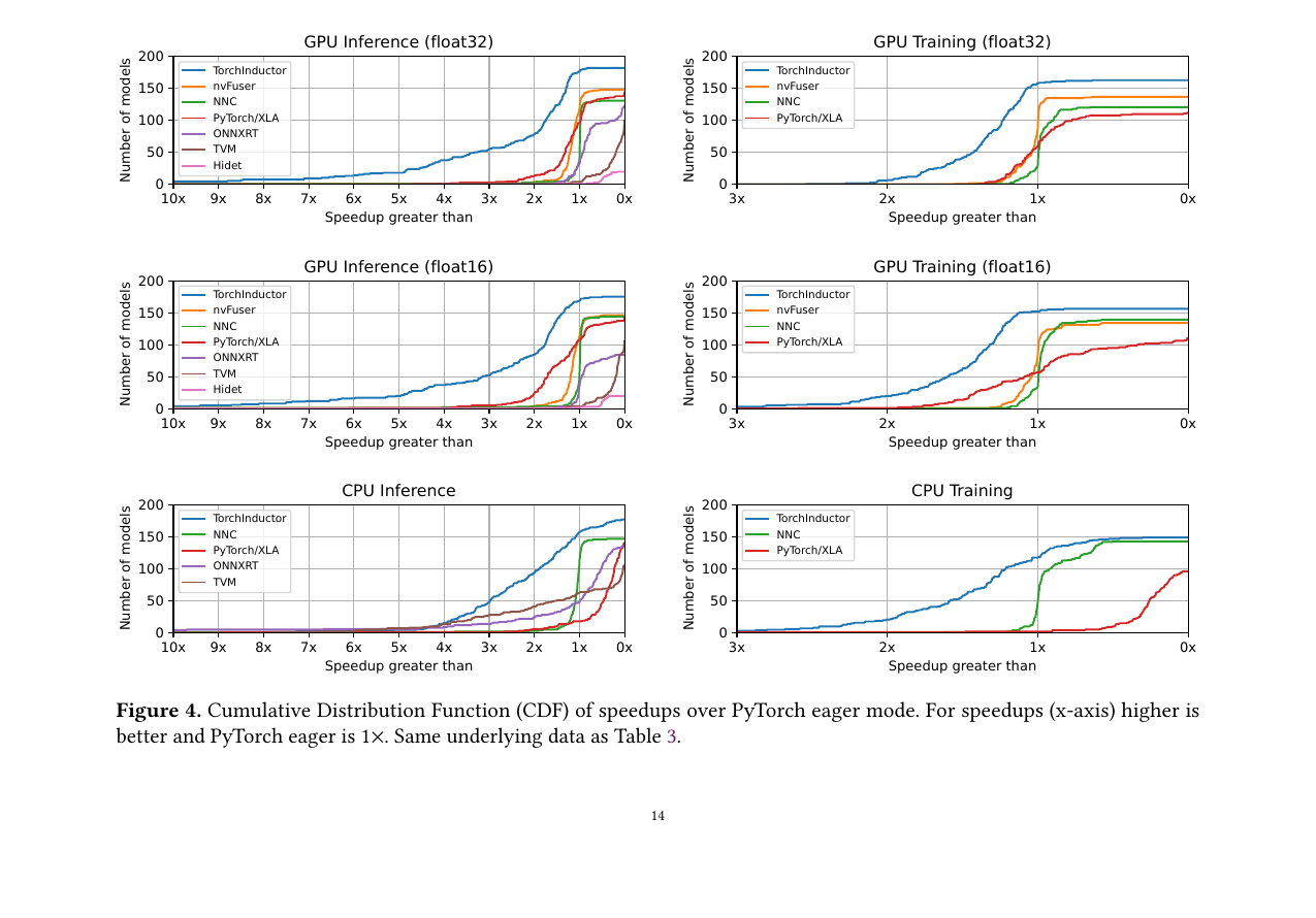
Figure 4 (Ansel et al., 2024): Cumulative Distribution Function of speedups over PyTorch eager mode across 180+ models from TorchBench, HuggingFace, and TIMM. TorchInductor (blue) dominates all other backends at every speedup threshold for both GPU inference (float32 and float16) and GPU training. The x-axis is inverted: curves further left indicate more models achieving higher speedups.
This is a survey of the full stack. Each stage has its own planned deep-dive: dynamo.md, aot-autograd.md, inductor.md, symbolic-shapes.md. The goal here is to establish the interfaces, invariants, and ordering rationale so that the deeper notes have a coherent home.
2. TorchDynamo: Python Bytecode Interception
🔑 TorchDynamo is the graph acquisition layer. Its job is to extract maximal sequences of PyTorch tensor operations from an arbitrary Python function into FX graph fragments, while generating guards that certify those fragments are valid for the current inputs.
2.1 The PEP 523 Frame-Eval Hook
CPython 3.6+ defines PEP 523, which allows a custom C-level callback to replace the default frame evaluation function (_PyEval_EvalFrameDefault). TorchDynamo calls set_eval_frame() to install its hook globally (scoped per-thread via a context manager when you call torch.compile).
Definition (Frame-Eval Hook). Let \(F\) denote a CPython execution frame — a struct containing the bytecode object (co_code), locals, the value stack, and the current instruction pointer. The hook function has the signature:
\[ \texttt{hook}(F, \texttt{throwflag}) \to \texttt{PyObject*} \]
When CPython is about to evaluate frame \(F\), it calls hook(F, 0) instead. Dynamo’s hook inspects whether \(F\) has already been compiled. If yes and guards pass, it replaces \(F\)’s code object with the compiled version and resumes normal evaluation. If no or guards fail, it calls _compile_frame(F).
sys.settrace or __torch_function__?
sys.settrace fires per Python line, not per bytecode instruction, and imposes enormous overhead. __torch_function__ only intercepts PyTorch operators — it misses Python control flow and non-tensor branches that affect graph structure. PEP 523 is the only hook that can intercept all computation at negligible cost.
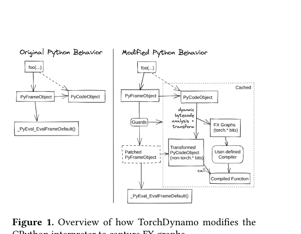
Figure 1 (Ansel et al., 2024): Side-by-side comparison of original CPython frame evaluation (left) and TorchDynamo’s modified behavior (right). On first call, Dynamo performs dynamic bytecode analysis to extract FX graph fragments, generates guards, and compiles a transformed PyCodeObject. On subsequent calls, the guard function is checked; if it passes, the cached compiled function is called directly, bypassing re-analysis.
2.2 Symbolic Bytecode Execution and Variable Trackers
_compile_frame runs the frame’s bytecode through InstructionTranslator, a symbolic interpreter. Rather than executing bytecode concretely, InstructionTranslator steps through each instruction and maintains a symbolic value stack where each slot holds a VariableTracker.
Definition (VariableTracker). A VariableTracker \(v\) is a runtime abstraction over a Python object. It carries:
- A source annotation (e.g., LocalSource("x")) recording where the object came from in the frame locals.
- A guard builder that knows what conditions must hold on the real object for this tracker to remain valid.
- Specialization-specific state depending on the Python type.
Key VariableTracker subtypes include TensorVariable (wraps a tensor; produces FX proxy nodes for operations), ConstantVariable (fully specializes a Python scalar or bool into the guard), ListVariable, TupleVariable, and UserDefinedObjectVariable (for objects Dynamo cannot specialize — treated opaquely, causing graph breaks if tensor-producing).
When InstructionTranslator encounters a bytecode instruction like BINARY_ADD, it calls the appropriate VariableTracker method (e.g., TensorVariable.__add__), which emits an FX call_function node into the OutputGraph and returns a new TensorVariable representing the result.
2.3 FX Graph Fragment Capture
The OutputGraph accumulates emitted FX nodes. When Dynamo reaches a point where it must stop (a graph break, a return, or fullgraph mode), it finalizes the graph into a torch.fx.GraphModule and passes it to the configured backend (by default, the aot_autograd wrapper over TorchInductor).
Suppose the original function has bytecode for y = torch.sin(x) + torch.cos(x). Dynamo rewrites the frame’s code object so that the executed bytecode instead calls __compiled_fn_0(x), where __compiled_fn_0 is the compiled FX graph. If a graph break occurs mid-function, a __resume_at_<offset> continuation function handles the remaining bytecode by recursively re-entering Dynamo.
The rewritten bytecode is cached: subsequent calls to the same function fast-path directly to the compiled code if guards pass, without re-entering _compile_frame.
2.4 Guard Generation
Guards are boolean predicates over the runtime inputs that certify a compiled graph fragment is valid. They are embedded as checks in the rewritten bytecode — evaluated before executing the compiled graph.
Definition (Guard). A guard \(g\) is a predicate \(g : \mathcal{I} \to \{\texttt{true}, \texttt{false}\}\) over the space \(\mathcal{I}\) of possible input values. If \(g(\mathbf{x}) = \texttt{true}\), the compiled code is correct for input \(\mathbf{x}\).
Guards are generated by GuardBuilder during symbolic bytecode execution. Each VariableTracker contributes guards appropriate to its type. Concrete examples:
| Guard type | What it checks | Generated by |
|---|---|---|
TENSOR_MATCH |
dtype, device, requires_grad, ndim | TensorVariable |
SIZE_MATCH |
concrete shape dimensions | TensorVariable (static mode) |
SHAPE_ENV |
symbolic inequality constraints | ShapeEnv (dynamic mode) |
EQUALS_MATCH |
Python scalar/bool value | ConstantVariable |
ID_MATCH |
object identity (e.g., a specific nn.Module instance) | ModuleVariable |
DISPATCH_KEY |
dispatch key bitset on tensor | TensorVariable |
DYNAMIC_INDICES |
which dimensions were seen with variable sizes | TensorVariable (dynamic mode) |
If a function branches on x.shape[0], Dynamo specializes the branch and records an EQUALS_MATCH guard on the concrete value. Every distinct value triggers a recompile. For shape-polymorphic code, use torch.compile(dynamic=True) to generate SHAPE_ENV inequalities instead.
2.5 Graph Breaks
A graph break occurs when InstructionTranslator encounters a construct it cannot trace inline:
- Calls to unsupported C extensions or arbitrary Python libraries.
- Tensor-to-Python data extraction:
x.item(),x.tolist(),bool(tensor). - Control flow that depends on a data-dependent boolean (e.g.,
if x.sum() > 0), unlesstorch.condis used. print,logging, or other side-effectful Python operations.torch.nn.Moduleforward methods with non-tensor state that Dynamo cannot model.
On a graph break, Dynamo:
1. Finalizes and compiles the FX fragment built so far.
2. Emits a __resume_at_<offset> bytecode stub that, when reached, restores the Python value stack and jumps to the instruction after the break point, recursively invoking Dynamo.
Each break prevents the backend compiler from seeing operations across the boundary. Cross-break fusion is impossible. In practice, a single break in a tight training loop can negate most of the speedup. Use torch.compile(fullgraph=True) to convert breaks into errors, making them visible during development.
This problem establishes how guards on either side of a graph break interact during recompilation.
Prerequisites: 2.4 Guard Generation, 2.5 Graph Breaks
A function f(x, n) contains a graph break triggered by print(n) where n is a Python integer. Dynamo compiles two FX fragments: \(G_1\) before the break and \(G_2\) after. Describe: (a) what guards are attached to each fragment, (b) what happens when f is called again with the same x but a different integer n, and (c) when it is called with the same n but a tensor x of different shape.
Key insight: Each compiled fragment has its own guard set. Guards for \(G_1\) cover the tensor properties of x (dtype, device, shape in static mode). Guards for \(G_2\) cover any properties of x that flow into \(G_2\) after the break. The integer n is accessed only inside the print call, which itself is the break-point; Dynamo does not trace through print, so n does not appear in either compiled fragment’s guards — it is simply executed eagerly.
Sketch:
- (a) \(G_1\)’s guards: dtype/device/shape of x. \(G_2\)’s guards: same properties of x (re-checked because \(G_2\) is entered through a new resume frame). n is not in any guard because it was consumed by the traced-over print.
- (b) Same x, different n: all guards pass (they don’t mention n). No recompile. The print(n) runs eagerly during the resume, printing the new value. Correct.
- (c) Same n, different x shape (static mode): SIZE_MATCH guard on \(G_1\) fails. Dynamo recompiles \(G_1\) (and likely \(G_2\), since x’s shape change may affect indexing). One new cache entry is added.
2.6 Recompilation Policy and Cache Structure
Each compiled Python function maintains a compilation cache — a linked list of (guard_fn, code_object) pairs. On each call:
- Dynamo evaluates
guard_fnfor each entry in order. - The first entry whose guards pass provides the
code_objectto execute. - If no entry passes,
_compile_frameis invoked: a new trace produces a new(guard_fn, code_object)pair appended to the list.
The cache is bounded: by default, Dynamo emits a warning after 8 recompilations for the same function and eventually stops compiling (falling back to eager) to avoid unbounded compile time. This threshold is configurable via torch._dynamo.config.cache_size_limit.
Separately from Dynamo’s per-frame cache, TorchInductor maintains a persistent FX Graph Cache keyed on a hash of the FX graph structure and guard values. If the same graph was compiled in a previous process run, Inductor can load the compiled artifact from disk, amortizing startup cost across process restarts.
3. The FX Intermediate Representation
Between Dynamo and AOTAutograd/Inductor, computation is represented as a torch.fx.GraphModule — PyTorch’s general-purpose program IR defined in Reed et al. (2022).
Definition (FX Graph). An FX graph \(\mathcal{G} = (V, E)\) is a directed acyclic graph where each vertex \(v \in V\) is an FX Node with:
- An opcode \(\in \{\texttt{placeholder}, \texttt{call\_function}, \texttt{call\_method}, \texttt{call\_module}, \texttt{get\_attr}, \texttt{output}\}\).
- A target: the function, method name, or module path being called.
- args and kwargs: edges to predecessor nodes or immediate Python values.
The six opcodes cover every pattern needed to represent PyTorch programs:
| Opcode | Semantics |
|---|---|
placeholder |
A function input (corresponds to def f(x, y, ...)) |
call_function |
Call a free Python/PyTorch function, e.g., torch.add |
call_method |
Call a method on a value, e.g., x.relu() |
call_module |
Invoke an nn.Module sub-module’s forward |
get_attr |
Read a parameter or buffer from the module hierarchy |
output |
The function’s return value(s) |
The entire graph is stored as an in-order list of Node objects (topological order by construction). Code generation reconstitutes executable Python by iterating this list and emitting calls.
Every stage — Dynamo output, AOTAutograd input/output, PrimTorch decomposition, Inductor input — uses FX graphs. Transformations are applied by graph-to-graph passes: a pass iterates nodes, replaces targets, inserts new nodes, and erases old ones — all in Python.
4. AOTAutograd: Ahead-of-Time Joint Tracing
💡 AOTAutograd sits between Dynamo and Inductor. It receives a forward FX graph, traces through PyTorch’s Autograd Engine to capture the backward graph before any data is seen at runtime, and hands a pair of functional FX graphs to the backend compiler.
4.1 Why Ahead-of-Time
In eager mode, the backward pass is built dynamically: each forward operator records a grad_fn node in the autograd tape, and .backward() traverses this tape at runtime. The compiler never sees the backward graph until it has already run.
AOTAutograd breaks this barrier. By tracing the backward graph ahead of time, it: - Makes both forward and backward graphs available simultaneously for cross-pass optimization. - Allows the backend to fuse backward kernels with each other and with forward epilogues. - Enables global decisions about which activations to save vs. recompute (rematerialization).
4.2 The Joint Forward-Backward Graph
Definition (Joint Graph). Given a user function \(f : \mathbb{R}^n \to \mathbb{R}^m\) (represented as an FX graph), AOTAutograd constructs a joint function:
\[ J(\mathbf{p}, \boldsymbol{\tau}) = (f(\mathbf{p}),\; \nabla_\mathbf{p} \langle f(\mathbf{p}), \boldsymbol{\tau} \rangle) \]
where \(\mathbf{p}\) are the primals (inputs and parameters) and \(\boldsymbol{\tau}\) are the tangents (upstream gradients). \(J\) returns both the forward outputs and the parameter gradients in a single graph.
The tracing mechanism uses make_fx — a function that applies torch.fx.Interpreter-based symbolic execution under __torch_dispatch__ to record operator calls as FX nodes. make_fx is invoked on the joint function with proxy tensors representing primals and tangents:
def joint_fn(primals, tangents):
    fw_outs = f(*primals)
    grads = torch.autograd.grad(fw_outs, primals, tangents)
    return fw_outs, grads

joint_graph = make_fx(joint_fn)(proxy_primals, proxy_tangents)
This is not standard FX symbolic tracing. Standard FX tracing uses __torch_function__ and does not see autograd. make_fx uses __torch_dispatch__, which fires after dispatch resolution — including through autograd — so both the forward operator calls and the backward AccumulateGrad / ViewBackward nodes are captured.
4.3 Functionalization
Backend compilers require pure functional graphs: no in-place mutation, no aliased tensors sharing storage. AOTAutograd applies functionalization to enforce this.
Definition (Functionalization). Functionalization is the transformation \(\phi\) that converts a graph with in-place operations and view aliases into a semantically equivalent pure functional graph. For each in-place op \(x \mathrel{+}= y\), \(\phi\) replaces it with \(x' = x + y\) and redirects all downstream uses of \(x\) to \(x'\).
Concretely, functionalization wraps tensors in FunctionalTensor objects. Mutations are recorded as functional shadow updates rather than applied to the underlying storage. After tracing, mutations are classified:
| Category | Meaning | Handling |
|---|---|---|
NOT_MUTATED |
Input unchanged | No action |
MUTATED_IN_GRAPH |
Mutation fully represented as a functional operation in the graph | Embedded in graph |
MUTATED_OUT_GRAPH |
Mutation cannot be expressed functionally within the trace | Applied via copy_() epilogue at runtime |
Similarly, view aliasing is resolved: the ViewAndMutationMeta structure tracks which outputs alias which inputs, and the runtime wrapper reconstructs the correct aliasing semantics after the functional graph executes.
4.4 Graph Partitioning via Min-Cut
After the joint graph is traced and functionalized, it must be split into a forward graph \(G_f\) and a backward graph \(G_b\). The forward graph saves certain intermediate tensors (saved activations) that the backward graph consumes.
The partition is a classic min-cut problem: minimize the bandwidth (total size of saved activations flowing from \(G_f\) to \(G_b\)) subject to the constraint that every value needed by \(G_b\) is either a primal input or a saved activation from \(G_f\).
Definition (Rematerialization). An activation \(a\) computed in \(G_f\) that is needed in \(G_b\) can either be saved (stored in memory, increasing peak activation memory) or recomputed (replicated in \(G_b\), increasing FLOPs). The min_cut_rematerialization_partition function applies a min-cut algorithm with the following heuristic edge weights:
\[ w(a) = \text{cost\_to\_save}(a) - \text{cost\_to\_recompute}(a) \]
Nodes with large memory footprint but cheap recomputation (e.g., relu, dropout) are candidates for recomputation. Expensive reductions (mean, sum over large tensors) are always saved. Views are always recomputed (zero compute cost).
torch.utils.checkpoint in eager mode is a runtime mechanism: it discards activations during the forward and re-runs the segment during backward. AOTAutograd’s rematerialization is a compile-time version of the same idea — more precise because the compiler can analyze the full graph rather than operating on user-specified segment boundaries.
4.5 Cross-Backward Fusion: What Eager Cannot Do
In eager mode, backward operators execute sequentially as the autograd engine traverses the tape. The kernel for SinBackward launches, completes, and writes its output to memory before AddBackward can begin. There is no opportunity for the two kernels to fuse.
With AOTAutograd, the backward graph \(G_b\) is a static FX graph. TorchInductor sees the entire backward at compile time and can fuse SinBackward and AddBackward into a single Triton kernel that reads inputs once, computes both gradients, and writes them back in one pass. This is the fundamental reason AOTAutograd exists: it lifts the backward graph from runtime-dynamic to compile-time-static.
This problem probes the boundary conditions of AOTAutograd’s tracing.
Prerequisites: 4.2 The Joint Forward-Backward Graph, 4.3 Functionalization
Consider a function f that contains a call to torch.linalg.solve(A, b). (a) Why does AOTAutograd have no difficulty tracing through this call? (b) Now suppose f calls a custom CUDA kernel written in C++ with no registered backward. What does AOTAutograd emit in the backward graph for this node, and what is the runtime consequence?
Key insight: AOTAutograd traces through __torch_dispatch__, which fires for any registered ATen operator. Custom CUDA kernels registered via TORCH_LIBRARY can have an autograd formula registered — in which case AOTAutograd captures it. If no formula is registered, the node becomes a dead end in the tape.
Sketch:
- (a) torch.linalg.solve is a standard ATen operator with a registered autograd formula. When make_fx traces the joint function, torch.autograd.grad invokes this formula under __torch_dispatch__, recording the backward ops (e.g., a matrix solve for the gradient of A) as FX nodes in the joint graph. No special treatment needed.
- (b) If the custom kernel has no setup_context/backward formula, torch.autograd.grad will raise RuntimeError: element 0 of tensors does not require grad and does not have a grad_fn. AOTAutograd will fail to trace the backward, and the entire torch.compile will fail for training. For inference (requires_grad=False), this is not an issue — AOTAutograd skips backward tracing entirely when no gradient is needed.
5. PrimTorch: Operator Decomposition
📐 PrimTorch addresses a fundamental portability problem: PyTorch exposes over 2,000 operator overloads at the ATen level (the C++ operator registry). Writing a compiler backend that correctly lowers all 2,000+ operators is impractical. PrimTorch solves this by decomposing ATen ops into a closed, stable set of ~250 primitive operators.
5.1 The Two Operator Levels
PrimTorch defines two distinct operator sets, both exposed under torch.ops.prims:
Definition (ATen ops). The ATen operator set consists of approximately 750 canonical operators (with ~2,000+ overloads counting dtype/layout variants). These are the operators visible at the Python-facing torch.* API. They have complex semantics (broadcasting, type promotion, view semantics, in-place variants) and are not all fusion-friendly. A backend targeting ATen ops must handle the full surface.
Definition (Prim ops). The prim operator set consists of approximately 250 primitive operators with simplified, stripped-down semantics: no type promotion rules, no broadcasting (inputs must have matching shapes), no in-place variants, and no aliasing. Each prim op corresponds to a tight loop-level computation that a compiler backend can directly map to hardware instructions.
The hierarchy is:
torch.* API (user-facing, ~2000 overloads)
     ↓ decomposes to
ATen ops (~750 canonical)
     ↓ decomposes to
Prim ops (~250 primitives)   ← compiler backends target this level
5.2 Decomposition at Trace Time
Decomposition happens as a graph transformation pass applied to the FX graph before it is handed to TorchInductor. The pass iterates every call_function node, checks if the target has a registered decomposition in torch._decomp.decompositions, and if so, replaces the node with its decomposition (an inline subgraph of more primitive ops).
Example. The ATen operator torch.nn.functional.gelu(x) decomposes as:
\[ \text{gelu}(x) = x \cdot \frac{1}{2}\left(1 + \text{erf}\left(\frac{x}{\sqrt{2}}\right)\right) \]
At the prim level, this becomes a sequence: prims.mul, prims.add, prims.erf, prims.sqrt, prims.div — all elementwise prims with no broadcasting or promotion semantics.
5.3 Why This Layer Exists
A new hardware vendor does not need to implement gelu, layer_norm, scaled_dot_product_attention, and 700 other ops. They implement the ~250 prims, and every ATen op decomposes into those prims at trace time. The compiler then fuses the resulting sequence of prims into efficient kernels for their hardware.
There is a deliberate tradeoff: decomposing gelu into five prims and then fusing them recovers the efficiency of a hand-fused gelu kernel — if the backend’s fusion engine is good enough. For backends without fusion (e.g., export to ONNX), it is better to target ATen ops directly and rely on the runtime to dispatch to vendor-optimized implementations.
This problem explores when decomposing to prims hurts performance.
Prerequisites: 5.1 The Two Operator Levels, 5.2 Decomposition at Trace Time
torch.nn.functional.layer_norm(x, normalized_shape, weight, bias) can decompose into prim ops (mean, variance, reciprocal sqrt, mul, add). TorchInductor fuses these back into a single kernel. However, cuDNN has a highly optimized cudnnLayerNormForward implementation that uses specialized memory access patterns TorchInductor’s Triton kernel cannot match. Describe the architectural mechanism by which TorchInductor can bypass the prim decomposition and call cuDNN directly for layer_norm.
Key insight: TorchInductor has its own lowering registry that maps ATen ops directly to hand-written Triton templates or external library calls, bypassing the prim decomposition path. The lowering registry takes priority over the generic decomposition → prim fusion path.
Sketch: Before applying prim decompositions, TorchInductor checks its internal lowering table for the ATen op. For aten.native_layer_norm, Inductor can register a lowering that emits a call to torch.ops.aten.native_layer_norm via the cuDNN path (or a custom Triton template). The decomposition to prims only fires for ops not in Inductor’s lowering table. This two-path design means frequently-used ops get optimized implementations while the long tail falls through to generic prim decomposition. The max-autotune mode extends this by also trying CUTLASS templates for mm/conv and benchmarking against the Triton-generated version.
6. TorchInductor: Loop-Level IR and Kernel Generation
🔑 TorchInductor is the default compiler backend. It receives a prim-level FX graph and produces optimized GPU (Triton) or CPU (C++/OpenMP) kernel code. Its core innovation is a define-by-run loop-level IR — a Python-native representation that enables both symbolic shape handling and straightforward code generation.
6.1 The Define-by-Run Loop IR
Definition (Inductor IR Node). An Inductor IR node for a pointwise operation is a Python callable of the form:
def inner_fn(index: list[sympy.Expr]) -> sympy.Expr:
    # index is a list of symbolic loop iteration variables
    # returns a symbolic expression for the output element at this index
    ...

node = torchinductor.ir.Pointwise(
    device=torch.device("cuda"),
    dtype=torch.float32,
    inner_fn=inner_fn,
    ranges=[size0, size1],   # symbolic loop bounds
)
The “define-by-run” terminology refers to the fact that the IR is not a static graph of nodes connected by edges. Instead, code generation is performed by executing inner_fn with symbolic index variables (SymPy Symbol objects), collecting the resulting symbolic expression, and then emitting the expression as Triton or C++ code.
For reductions, the analogous structure is torchinductor.ir.Reduction, which has both an inner_fn (computing the element to reduce over) and a reduction_fn (the accumulation, e.g., sum or max).
Key property: The Inductor IR is lazy. An ir.Pointwise node does not compute anything; it only becomes concrete when the scheduler decides to emit it as a kernel and calls inner_fn with the iteration variables.
6.2 Symbolic Shapes with SymPy
Static-shape compilation — where every tensor dimension is a concrete integer — yields optimal loop bounds and enables loop tiling decisions to be made at compile time. But it produces a separate compiled artifact for every distinct input shape, leading to cache thrashing for transformer models with variable sequence lengths.
TorchInductor uses SymPy to represent symbolic shapes: dimension values are sympy.Symbol objects (e.g., s0, s1) that flow through all indexing arithmetic. A compiled Triton kernel with symbolic shapes contains runtime-computed index expressions:
# Generated Triton kernel (schematic) for a pointwise op on shape [s0, s1]
@triton.jit
def kernel(x_ptr, out_ptr, s0, s1, ...):
    pid = tl.program_id(0)
    offset = pid * BLOCK_SIZE + tl.arange(0, BLOCK_SIZE)
    mask = offset < s0 * s1
    x = tl.load(x_ptr + offset, mask=mask)
    tl.store(out_ptr + offset, tl.sin(x), mask=mask)
At runtime, s0 and s1 are passed as kernel arguments. The kernel is correct for any values satisfying the guard inequalities established during compilation (e.g., \(s_0 > 0\), \(s_1 > 0\)).
SymPy handles the algebra: it simplifies expressions like s0 * s1 + s0 * 0 to s0 * s1, eliminates redundant index terms from strides, and generates readable guard predicates.
By default, TorchInductor specializes on \(s = 0\) and \(s = 1\) even in dynamic mode. A zero-size tensor requires a boundary check that would complicate the general case; a size-one tensor often enables broadcast elimination. Every other size is treated symbolically.
6.3 The Scheduler and Fusion
The Inductor Scheduler is the component that decides which IR nodes are fused into the same kernel. Its decisions directly control memory traffic: two fused pointwise nodes share a single HBM read/write cycle; unfused nodes each pay independently.
Definition (Fusion Categories). The scheduler partitions IR nodes into three categories:
- Pointwise: elementwise operations (sin, add, mul, relu, …). Any two pointwise nodes with compatible iteration domains can fuse.
- Reduction: operations that reduce along one or more dimensions (sum, max, mean). A reduction can fuse with preceding pointwise ops that feed it, but two reductions cannot fuse with each other (they would require nested loops with incompatible structure).
- Template: pre-written Triton or CUTLASS kernels for matmul and conv. Templates fuse with succeeding pointwise ops (epilogue fusion) but not with preceding reductions.
Fusion decisions are scored by estimated memory traffic reduction:
\[ \Delta_{\text{traffic}}(A \cup B) = \text{traffic}(A) + \text{traffic}(B) - \text{traffic}(A \cup B) \]
A fusion is performed if \(\Delta_{\text{traffic}} > 0\). The scheduler also checks iteration domain compatibility: two nodes can fuse only if their loop ranges are identical or one can be broadcast into the other.
6.4 GPU Path: Triton Codegen
For GPU targets, the scheduler’s fusion groups are lowered to Triton kernels. Triton is a Python-embedded DSL for writing GPU kernels at the tile level — the programmer specifies tile sizes and the compiler handles CUDA thread-block mapping, shared memory, and vectorization.
Inductor’s code generator calls each fused node’s inner_fn with symbolic Triton tile indices (SymPy expressions quantized to tl.arange expressions) and collects the resulting symbolic tree. It then emits Triton source by recursively printing the tree:
| Inductor op | Triton emission |
|---|---|
prims.sin |
tl.sin(...) |
prims.add |
... + ... |
prims.load |
tl.load(ptr + idx, mask=mask) |
prims.store |
tl.store(ptr + idx, val, mask=mask) |
| Reduction sum | tl.sum(...) |
For matmul and conv, Inductor uses template kernels: pre-written Triton code for the matrix multiply loop, with a user-supplied epilogue insertion point. The template produces a MultiTemplate buffer holding \(N\) candidate GEMM implementations (different tile sizes, different pipelining depths). In max-autotune mode, the scheduler benchmarks all candidates and picks the fastest.
Epilogue fusion. After selecting the GEMM winner, the scheduler checks whether any immediately-downstream pointwise ops (e.g., bias_add, gelu, dropout) can be inlined into the GEMM’s output tile before it is written back to HBM. This epilogue fusion eliminates one round of HBM traffic: the GEMM output never materializes as a full tensor.
6.5 CPU Path: C++ and OpenMP
For CPU targets, the same IR is lowered to C++ loops with #pragma omp parallel for annotations. The scheduler still performs fusion, and symbolic shape expressions become C++ variable references. The generated code is compiled at runtime via the system C++ compiler (typically GCC or Clang) and loaded as a shared library.
CPU code generation benefits from the same symbolic shape machinery: a single compiled artifact handles variable batch sizes without recompilation.
6.6 Layout Propagation
PyTorch tensors can have contiguous (row-major, NCHW) or channels-last (NHWC) memory layout. Many convolution workloads are faster in channels-last format because it exposes more contiguous memory accesses along the channel dimension, which maps better to GPU vectorized loads.
However, naively inserting layout conversions at every operator boundary is expensive. TorchInductor performs layout propagation: it analyzes the graph and determines a global layout assignment that minimizes conversion overhead. Operations like conv2d prefer channels-last; operations like linear are layout-agnostic. The scheduler assigns layouts and inserts permute/contiguous nodes only where conversions are unavoidable.
This problem establishes why two reductions cannot fuse into a single kernel.
Prerequisites: 6.3 The Scheduler and Fusion, 6.4 GPU Path: Triton Codegen
Let \(A\) be a sum reduction over the column dimension of a matrix \(X \in \mathbb{R}^{M \times N}\) (yielding a vector in \(\mathbb{R}^M\)) and \(B\) be a sum reduction over the row dimension of \(X\) (yielding a vector in \(\mathbb{R}^N\)). Both \(A\) and \(B\) read from \(X\). Prove that \(A\) and \(B\) cannot be fused into a single Triton kernel without producing an incorrect result or incurring the same memory traffic as two separate kernels.
Key insight: \(A\) and \(B\) have incompatible iteration domains and reduction axes. Fusing them requires a thread block to simultaneously reduce along rows and columns — which requires either processing the full matrix twice (no saving) or a two-phase reduction that is strictly more expensive than two separate passes.
Sketch: In Triton, a reduction kernel assigns program IDs to output elements. For \(A\) (column sum), each program ID corresponds to one row of \(X\), and the kernel accumulates over columns. For \(B\) (row sum), each program ID corresponds to one column, and the kernel accumulates over rows. To fuse, we would need each thread block to handle both a row-accumulation and a column-accumulation — but the memory access pattern for rows (strided) and columns (contiguous) require different tile geometries. Any fusion must either: (1) materialize \(X\) into shared memory twice (one per reduction direction), paying the same HBM bandwidth as two kernels; or (2) assign different thread block structures to the two reductions, which is equivalent to two separate kernel launches. The scheduler’s iteration-domain compatibility check correctly blocks this fusion.
7. End-to-End Data Flow
The diagram below traces a single call to a torch.compiled function f(x) from Python invocation through to GPU kernel launch, showing the artifact produced at each stage boundary.
flowchart TD
    A["Python call: compiled_f(x)"] --> B{"Guard check
passes?"}
    B -->|"yes"| C["Execute cached
compiled code object"]
    B -->|"no / first run"| D["Dynamo: _compile_frame(F)"]

    D --> E["InstructionTranslator
symbolic bytecode execution"]
    E --> F["OutputGraph accumulates
FX nodes (ATen level)"]
    F --> G["Guard generation
(GuardBuilder)"]
    G --> H["FX GraphModule
(ATen ops, placeholder/call/output nodes)"]

    H --> I["AOTAutograd
make_fx joint tracing"]
    I --> J["Functionalization
in-place ops removed"]
    J --> K["min_cut partition"]
    K --> L["Forward FX GraphModule
+ Backward FX GraphModule"]

    L --> M["PrimTorch decomposition pass
ATen ops -> prim ops"]
    M --> N["Prim-level FX GraphModule
(~250-op surface)"]

    N --> O["Inductor lowering
FX nodes -> IR nodes (Pointwise / Reduction / Template)"]
    O --> P["Scheduler
fusion decisions, layout propagation"]
    P --> Q{"GPU or CPU?"}

    Q -->|"GPU"| R["Triton codegen
inner_fn + SymPy -> .py source"]
    Q -->|"CPU"| S["C++/OpenMP codegen
inner_fn -> .cpp source"]

    R --> T["triton.compile()"]
    S --> U["g++ / clang compile"]

    T --> V["Compiled CUDA kernel (.cubin)"]
    U --> W["Shared library (.so)"]

    V --> X["Kernel launch: device execution"]
    W --> X

    C --> X
Stage boundaries summarized:
| Handoff | From | To | Artifact |
|---|---|---|---|
| Dynamo → AOTAutograd | Frame-eval hook | aot_module wrapper |
torch.fx.GraphModule at ATen level |
| AOTAutograd → Decomp | make_fx + functionalize |
Decomposition pass | Functional GraphModule, ATen level |
| Decomp → Inductor | Decomposition pass | Inductor lowering | Prim-level GraphModule |
| Inductor lowering → Scheduler | lower_to_ir() |
Scheduler |
Pointwise/Reduction/Template IR nodes |
| Scheduler → Codegen | Fusion grouping | TritonKernel / CppKernel |
Python Triton source / C++ source |
| Codegen → Runtime | triton.compile() / gcc |
Kernel cache | .cubin / .so |
8. Guards and Recompilation in Depth
8.1 Guard Types
Guards are the contract between Dynamo’s compiled artifact and the runtime input. They are embedded in the rewritten bytecode as a sequence of Python boolean checks. If any guard fails, the cache miss handler triggers recompilation.
The full taxonomy of guard types, ordered roughly from cheapest to most expensive to evaluate:
| Guard | Cost | Triggered by |
|---|---|---|
EQUALS_MATCH on Python scalar |
O(1) comparison | Python int/float/bool used in the graph |
ID_MATCH on object |
O(1) identity check | nn.Module instance, Python object |
TENSOR_MATCH on dtype/device |
O(1) attribute read | Any tensor input |
TENSOR_MATCH on requires_grad |
O(1) | Any tensor input |
SIZE_MATCH on concrete shape |
O(rank) | Static shape mode |
DISPATCH_KEY bitmask check |
O(1) | Tensor dispatch key set |
SHAPE_ENV inequality |
O(num constraints) | Dynamic shape mode |
DYNAMIC_INDICES attribute |
O(ndim) | Mixed static/dynamic dimension mode |
8.2 Cache Lookup Mechanism
Definition (Compilation Cache Entry). An entry \(e_i = (g_i, c_i)\) in Dynamo’s per-function cache consists of:
- \(g_i\): a guard function g_i(L) -> bool where L is the frame locals dictionary.
- \(c_i\): a Python code object to execute if \(g_i\) passes.
On a call to the compiled function:
for (guard_fn, code_obj) in cache:
    if guard_fn(frame.locals):
        exec(code_obj, frame.globals, frame.locals)
        return
# cache miss:
new_entry = compile_frame(frame)
cache.append(new_entry)
exec(new_entry.code_obj, ...)
The linear scan is \(O(|\text{cache}|)\), bounded by cache_size_limit (default 8). In practice, caches rarely exceed 2–3 entries for well-structured code.
8.3 Specialization vs. Dynamic Shapes
torch.compile exposes a dynamic parameter controlling how Dynamo handles shape variability:
Static specialization (dynamic=False, default). Every tensor dimension is matched concretely. A new batch size triggers a recompile, producing a new entry in the cache. This yields maximally optimized kernels (loop bounds are compile-time constants, enabling aggressive unrolling and tile-size selection) but causes cache thrashing with variable-length inputs.
Dynamic shapes (dynamic=True). Dynamo assigns sympy.Symbol objects to tensor dimensions that have been seen with different values, and records SHAPE_ENV guards encoding the observed constraints (e.g., \(s_0 \geq 1\), \(s_0 \leq 2048\)). The compiled Triton kernel receives shape values as runtime arguments and handles any conforming size without recompilation.
Surprisingly, dynamic shape compilation often incurs only a 5–10% overhead relative to static compilation — the SymPy symbolic expressions in Triton kernels typically optimize to the same code as if the bounds were constant, because Triton’s LLVM backend eliminates the symbolic parameter once it is known at kernel-call time.
dynamic=True does not make all dimensions symbolic. Dimensions that are always seen with the same value remain specialized. Dynamo uses the DYNAMIC_INDICES mechanism to track, per-tensor, which dimensions have been observed with variable sizes — only those become symbols. This is the mark_dynamic / mark_static API.
This problem analyzes the amortized cost of guard evaluation for a high-throughput inference server.
Prerequisites: 8.1 Guard Types, 8.2 Cache Lookup Mechanism
A production inference service calls compiled_model(x) at 10,000 requests/second. Each call evaluates 12 guards (all TENSOR_MATCH type, 4 ns each). The compiled kernel itself takes 500 µs to execute. (a) What fraction of total per-call time is spent on guard evaluation? (b) The team considers switching to reduce-overhead mode (CUDA graphs). What does CUDA graph capture do to guard evaluation overhead, and what constraint does it impose on inputs?
Key insight: Guard evaluation is negligible relative to kernel execution in the high-throughput case, but CUDA graphs eliminate even that overhead at the cost of fixed input/output addresses.
Sketch:
- (a) Guard time per call: \(12 \times 4\,\text{ns} = 48\,\text{ns}\). Kernel time: \(500\,\mu\text{s} = 500{,}000\,\text{ns}\). Guard fraction: \(48 / 500{,}048 \approx 0.0096\%\). Negligible.
- (b) CUDA graphs capture the entire sequence of CUDA API calls (kernel launches, memory ops) into a replay graph. After capture, a single cudaGraphLaunch replays all operations without re-issuing individual CUDA calls, eliminating Python overhead and CPU-side kernel launch latency. However, CUDA graphs require that tensor addresses and shapes are fixed at capture time — the graph is recorded for specific pointer values. This means inputs must be placed in pre-allocated, fixed-address buffers. Variable-length inputs (different sequence lengths) require either padding to a fixed size or maintaining separate CUDA graphs per shape, increasing memory usage.
9. torch.compile Usage Modes
torch.compile accepts a mode string that selects a preset combination of Inductor compiler flags:
compiled_model = torch.compile(
    model,
    mode="default",        # or "reduce-overhead", "max-autotune", "max-autotune-no-cudagraphs"
    dynamic=False,         # True for dynamic shapes
    fullgraph=False,       # True to raise on any graph break
    backend="inductor",    # or "eager", "aot_eager", or custom
)| Mode | CUDA Graphs | Autotuning | Compile Time | Best For |
|---|---|---|---|---|
"default" |
No | No | Low | General use; first deployment |
"reduce-overhead" |
Yes | No | Low | Small models on large GPUs; Python-bound inference |
"max-autotune" |
Yes | Yes (GEMM, conv) | High | Throughput-critical inference; large batch training |
"max-autotune-no-cudagraphs" |
No | Yes | High | Variable-shape inputs needing best kernel selection |
"default" applies the standard Inductor pipeline: prim decomposition, scheduler fusion, Triton/C++ codegen, symbolic shapes if dynamic=True. No autotuning — the first tile configuration tried is used. Compile time is typically 30–120 seconds for a large model on first run.
"reduce-overhead" enables CUDA graph capture. After the first few warmup runs (to populate caches and let Dynamo stabilize), Inductor captures a CUDA graph: a recording of all CUDA API calls for one forward pass. Subsequent calls replay the graph with a single cudaGraphLaunch, eliminating Python-side overhead and per-kernel-launch CPU cost. This can be 2–5× faster for small models where Python overhead dominates. The constraint is fixed input tensor addresses and shapes.
"max-autotune" enables CUDA graphs and exhaustive autotuning. For matmul and conv nodes, Inductor generates \(N\) candidate Triton templates (varying tile sizes \(M_t \times N_t \times K_t\), number of pipeline stages, and split-k configurations) and benchmarks each on the target hardware. It selects the fastest and caches the winner. This adds significant compile time (minutes for a large model) but produces hardware-optimal kernels. On A100, autotune can recover 10–30% performance over default for GEMM-heavy workloads.
"max-autotune-no-cudagraphs" provides autotuning without the fixed-address constraint, suitable for models with variable-length inputs (e.g., language model inference with dynamic sequence length).
backend parameter
Setting backend="eager" runs Dynamo without any compilation — useful for debugging guard logic and graph breaks. backend="aot_eager" adds AOTAutograd tracing (capturing the joint graph) but skips Inductor — useful for testing AOTAutograd correctness. Custom backends are functions (fx.GraphModule, example_inputs) -> Callable.
This problem identifies a common failure mode when combining CUDA graphs with dynamic-allocation patterns.
Prerequisites: 9. torch.compile Usage Modes, 8.3 Specialization vs. Dynamic Shapes
A model uses torch.where(mask, x, torch.zeros_like(x)) where mask is a boolean tensor that varies at runtime. A colleague says: “I switched to reduce-overhead mode and my outputs are now always zeros on the second call.” Explain the mechanism of this bug and the correct fix.
Key insight: CUDA graphs capture tensor addresses, not tensor contents. If the model allocates a new torch.zeros_like(x) tensor on every call, the CUDA graph replay re-uses the captured address — which now points to a stale allocation, potentially deallocated and reallocated for a different tensor.
Sketch: During CUDA graph capture (warmup run), torch.zeros_like(x) allocates a buffer at address \(A_0\), filled with zeros. The CUDA graph records a cudaMemcpyAsync from \(A_0\) in the torch.where kernel. On replay, the graph issues the same copy from \(A_0\), but if the allocator has reused \(A_0\) for another tensor (e.g., an intermediate activation), the values at \(A_0\) are no longer zeros. Fix: pre-allocate the zeros buffer outside the compiled function and pass it as an explicit input (so it has a stable address captured in the graph), or use torch.compile(mode="max-autotune-no-cudagraphs") to disable CUDA graphs. Alternatively, replace the pattern with x * mask (a pure elementwise op with no dynamic allocation) which compiles cleanly under CUDA graphs.
References
| Reference | Brief Summary | Link |
|---|---|---|
| Ansel et al., “PyTorch 2: Faster ML Through Dynamic Python Bytecode Transformation” (ASPLOS 2024) | Primary source for the full torch.compile stack; covers Dynamo frame-eval hook, AOTAutograd, PrimTorch, Inductor, and benchmark results | dl.acm.org |
| Jason Ansel, “TorchDynamo: An Experiment in Dynamic Python Bytecode Transformation” (dev-discuss, 2022) | Original TorchDynamo design doc; bytecode analysis rationale, guard structure, FX fragment capture | dev-discuss.pytorch.org |
| Jason Ansel, “TorchInductor: a PyTorch-native Compiler with Define-by-Run IR” (dev-discuss, 2022) | Inductor design: define-by-run IR, SymPy symbolic sizes, Triton GPU path, epilogue fusion | dev-discuss.pytorch.org |
| Reed et al., “torch.fx: Practical Program Capture and Transformation for Deep Learning in Python” (MLSys 2022) | Defines the FX IR (GraphModule, Node, opcodes) that all torch.compile stages use | arxiv.org/abs/2112.08429 |
| PyTorch, “Dynamo Overview” (official docs, 2024) | Authoritative reference for frame-eval hook, guard types, recompilation policy, cache structure | docs.pytorch.org |
| PyTorch, “AOT Autograd: How to use and optimize?” (functorch docs) | AOTAutograd joint graph tracing, partitioning, and cross-backward fusion examples | docs.pytorch.org/functorch |
| PyTorch, “Introduction to torch.compile” (tutorial) | End-to-end usage guide; fullgraph parameter, graph break detection | docs.pytorch.org |
| Modal, “What do the parameters of torch.compile do?” (blog, 2024) | Concise reference for mode, dynamic, fullgraph, and backend parameters |
modal.com |
| DeepWiki, “TorchDynamo” (pytorch/pytorch) | Architectural walkthrough of InstructionTranslator, VariableTrackers, OutputGraph, and ShapeEnv | deepwiki.com |
| DeepWiki, “AOT Autograd and Functionalization” (pytorch/pytorch) | Detailed treatment of joint tracing, FunctionalTensor, mutation classification, and min-cut partitioning | deepwiki.com |
| Ian Barber, “Inductor Notes” (blog, 2024) | Practical notes on Inductor scheduling, fusion scoring, Triton emission, and autotuning | ianbarber.blog |
| PyTorch, “torch.compile API reference” (stable docs) | Full API documentation for torch.compile parameters |
docs.pytorch.org |