🔬 torch.fx: Practical Program Capture and Transformation
Reed, DeVito, He, Ussery, Ansel — MLSys 2022 (arXiv 2112.08429)
Table of Contents
- 1. Motivation: The Eager–Graph Tension
- 2. Background: The Design Space
- 3. Design Principles
- 4. Program Capture: Symbolic Tracing
- 5. The IR: Graph, Node, and GraphModule
- 6. Source-to-Source Code Generation
- 7. Design Decisions
- 8. Writing Graph Transforms
- 9. Case Studies
- References
1. Motivation: The Eager–Graph Tension
PyTorch’s eager execution model is excellent for development: every operator dispatches immediately through the C10 Dispatcher, results are available for inspection at any Python breakpoint, and pdb works out of the box. But eager mode has a structural limitation — the runtime only ever sees one operator at a time. This precludes a class of transformations that require non-local program context:
| Transform | What it needs to see |
|---|---|
| Operator fusion | Two adjacent ops simultaneously, to merge their kernels |
| Quantization | The activation tensor produced by one op and consumed by the next |
| Conv–BN fusion | A Conv2d node and the immediately-following BatchNorm2d node |
| Device lowering | The entire computation graph to schedule onto a fixed-memory accelerator |
| FLOP counting / shape prop | The complete DAG with all tensor shapes |
To apply any of these transforms, you need to capture the program structure — inspect it as a data structure before running it. This is the gap torch.fx fills.
The key insight: most neural networks are basic block programs — flat sequences of tensor operations with no data-dependent control flow (no if tensor_value > 0, no dynamic loops). For this majority case, a deliberately simple IR suffices, and building for the majority makes the system far easier to use and implement than TorchScript’s full-Python model.
2. Background: The Design Space
2.1 Capturing Program Structure
The paper identifies three approaches to program capture:
Concrete tracing (torch.jit.trace): run the program on real inputs, record which ops fire. Simple to implement, but incidentally shape-specializes — a jit.trace with batch size 4 produces a graph that is incorrect for batch size 8 if any shape-dependent control flow was exercised.
Symbolic tracing (torch.fx, MXNet Gluon, tf.function): run the program with abstract proxy values rather than real tensors. No concrete shapes flow through, so no accidental specialization. Fails silently on data-dependent control flow (e.g. if x.sum() > 0) — but this failure is observable and raises an error in torch.fx.
Embedded language compilation (TorchScript): parse the Python source with a full lexer–parser–compiler toolchain. Supports richer programs including control flow and user-defined types. High complexity to implement and to write transforms against: TorchScript’s ResNet IR has 2614 nodes from jit.script vs. 445 for torch.fx.
torch.fx chooses symbolic tracing for its simplicity, and makes the limitations configurable rather than trying to handle the long tail.
2.2 Specializing Programs
Specialization means committing to specific values (shapes, dtypes, Python scalars) at capture time. More specialization → smaller, faster artifacts; less generality.
- Shape specialization (
jit.trace): committed to specific shapes. Wrong for other shapes. - JIT specialization (LazyTensor, DyNet): capture on every invocation, then apply transforms and cache. Correct for all inputs but pays capture overhead repeatedly.
- AoT without specialization (torch.fx): capture once ahead-of-time. The IR contains no specialization — it is the transform’s job to decide what to specialize, if anything. Predictable and observable, at the cost of not handling input-dependent control flow.
2.3 Intermediate Representation Design
Three axes of IR design:
Language: Protocol Buffers (TensorFlow), C++ data structures (TorchScript), Python objects (torch.fx). torch.fx chooses Python — transforms are written in Python and can be debugged with pdb.
Control flow: Most ML models are basic block programs (MLPs, CNNs, Transformers without decoder loops). Representing control flow in the IR forces every analysis to be a fixpoint dataflow computation — expensive to implement correctly, even for compiler writers. torch.fx omits control flow entirely.
For a basic block, shape analysis is a single forward pass: iterate nodes in topological order, propagate shapes through each operator. With a loop in the IR, shape analysis is a fixpoint computation: iterate until convergence, because a loop-carried tensor can take infinitely many shapes depending on iteration count (e.g. torch.cat in a loop). torch.fx avoids this entirely by not representing loops.
State (mutability): PyTorch tensors support aliasing (x[i] is a view of x) and in-place mutation (x[i] = y). Reasoning about mutation safety requires alias analysis — annotating every op with aliasing semantics and running a points-to analysis. torch.fx treats mutation as undefined behavior and raises an error if captured. Model parameters live in the stateful GraphModule, cleanly separated from the functional Graph.
3. Design Principles
The paper states three principles that drive torch.fx’s design:
Prefer correctness for typical models over generality. torch.fx will fail on models with data-dependent control flow. This is acceptable because the failure is explicit (an error with a stack trace), and the vast majority of production models don’t need it.
Work within the Python ecosystem. IR is Python objects. Transforms are Python functions. Output is Python code. ML practitioners don’t need to learn Protocol Buffers or C++.
Make capture configurable. Long-tail problems are handled by subclassing
Tracer, not by complicating the core system. Users can block tracing into specific submodules (is_leaf_module), install metadata on nodes (create_proxy), or specialize on tensor metadata they care about.
4. Program Capture: Symbolic Tracing
The paper’s overview figure shows the full pipeline at a glance: symbolic_trace captures a function into a Graph of Node objects, then regenerates executable Python code from that graph.
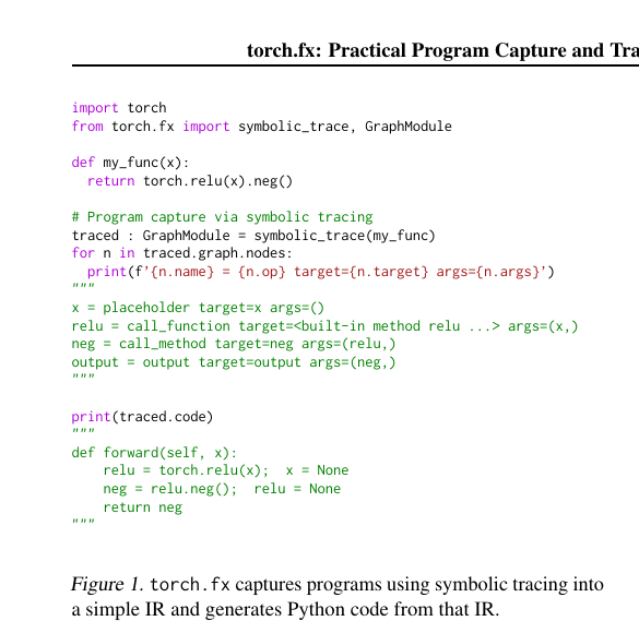
Figure 1 (Reed et al., 2022): torch.fx captures programs via symbolic tracing into a six-opcode IR and regenerates Python code from that IR. The call_function node holds a direct reference to the Python callable; call_method records method calls on the first argument.
4.1 The Proxy Data Structure
Symbolic tracing works by substituting every input tensor with a Proxy — a duck-typed Python object that records operations on it instead of executing them.
Definition (Proxy). A Proxy is a Python object that:
- Intercepts attribute access (proxy.shape, proxy.dtype) and method calls (proxy.relu()) by recording them as Node objects in a Graph.
- Implements __torch_function__ to intercept free PyTorch functions (torch.add(a, b), torch.sin(x)).
- Returns another Proxy from any operation, so the substitution propagates forward through the entire function.
Here is a minimal implementation that captures the core idea:
class MiniGraph:
    def __init__(self):
        self.nodes: list[dict] = []

    def add_node(self, op, target, args=(), kwargs=None):
        name = f"{target.__name__ if callable(target) else target}_{len(self.nodes)}"
        node = {"name": name, "op": op, "target": target, "args": args, "kwargs": kwargs or {}}
        self.nodes.append(node)
        return node


class MiniProxy:
    """
    Records operations into a Graph instead of executing them.
    Returns self (another Proxy) from every operation so the substitution
    propagates through the traced function.
    """
    def __init__(self, node: dict, graph: MiniGraph):
        self.node = node
        self.graph = graph

    def __add__(self, other):
        node = self.graph.add_node(
            op="call_function",
            target=lambda a, b: a + b,  # stand-in for torch.add
            args=(self.node["name"], _node_name(other)),
        )
        return MiniProxy(node, self.graph)

    def relu(self):
        node = self.graph.add_node(
            op="call_method",
            target="relu",
            args=(self.node["name"],),
        )
        return MiniProxy(node, self.graph)

    def __repr__(self):
        return f"Proxy({self.node['name']})"


def _node_name(x):
    return x.node["name"] if isinstance(x, MiniProxy) else x


def mini_trace(fn, *input_names):
    graph = MiniGraph()
    proxies = []
    for name in input_names:
        node = graph.add_node("placeholder", name)
        proxies.append(MiniProxy(node, graph))
    output = fn(*proxies)
    graph.add_node("output", "output", args=(output.node["name"],))
    return graph


def my_fn(x, y):
    return (x + y).relu()


graph = mini_trace(my_fn, "x", "y")
for n in graph.nodes:
    print(n["op"], n["target"] if isinstance(n["target"], str) else "<fn>", n["args"])

# placeholder x ()
# placeholder y ()
# call_function <fn>  ('x_0', 'y_1')
# call_method   relu  ('<fn>_2',)
# output        output ('<fn>_2_relu_3',)  # (names simplified)
The real torch.fx.Proxy does the same thing, but also implements __torch_function__, __getattr__ for tensor attributes, and wraps the full ATen operator surface.
This problem establishes when symbolic substitution breaks down.
Prerequisites: 4.1 The Proxy Data Structure
A function f(x) contains the line if x.shape[0] > 1: return x * 2. When f is symbolically traced with a MiniProxy substituted for x, what happens when Python evaluates the if statement, and why does this constitute a fundamental limitation of symbolic tracing rather than a bug in the implementation?
Key insight: if requires a concrete Python bool. x.shape[0] on a Proxy returns another Proxy (the shape is symbolic). Proxy > 1 would return a Proxy. Python’s if then calls bool(proxy), which cannot produce a meaningful boolean — it raises a torch.fx.proxy.TraceError. This is not a bug: the information needed to resolve the branch (the actual value of x.shape[0]) does not exist at trace time. The Proxy has no concrete data. Fixing this would require either (a) concrete specialization (losing generality) or (b) lifting the if into a graph node (requiring control flow in the IR — the complexity torch.fx deliberately avoids).
4.2 The Tracer and __torch_function__
The real torch.fx symbolic tracer uses two interception mechanisms:
__torch_function__— a Python protocol on tensor subclasses. When a free PyTorch function (e.g.torch.relu,torch.add) is called with an argument that implements__torch_function__, PyTorch callstype(arg).__torch_function__(func, types, args, kwargs)instead of executingfunc.Proxyimplements this to recordcall_functionnodes.Module override —
Tracer.call_moduleis invoked when acall_modulenode should be recorded (i.e. when a tracednn.Module.forwardcalls a sub-module).
Here is a minimal __torch_function__ implementation:
import torch

class TracingProxy(torch.Tensor):
    """
    A Tensor subclass that records operations into a graph.
    __torch_function__ fires for all torch.* free functions.
    """
    _graph: list  # class-level graph accumulator (simplified)

    @classmethod
    def __torch_function__(cls, func, types, args=(), kwargs=None):
        kwargs = kwargs or {}
        # Record the call instead of executing it
        node = {"op": "call_function", "target": func, "args": args, "kwargs": kwargs}
        cls._graph.append(node)
        # Return another TracingProxy so the substitution propagates
        result = cls.__new__(cls)
        result._node = node
        return result
The real torch.fx.Proxy is not a Tensor subclass — it uses __torch_function__ via a wrapper but is a plain Python object. The above simplification illustrates the interception mechanism.
Definition (Tracer). The Tracer class controls the symbolic tracing process. Its two most important overridable methods are:
is_leaf_module(m, qualname) -> bool— returnsTrueif a sub-module should be treated as an opaquecall_modulenode (not traced into). Default: built-innnmodules likenn.Conv2dare leaves; user-defined modules are traced through.create_proxy(kind, target, args, kwargs) -> Proxy— called whenever a newNodeand its associatedProxyare about to be created. Can be overridden to attach metadata.
4.3 Configurable Capture via Tracer Subclassing
The paper emphasizes that edge cases are handled by subclassing Tracer, not by complicating the core.
import torch.fx as fx

class ShapeAwareTracer(fx.Tracer):
    """
    A Tracer that also records the concrete shape of each tensor
    on the corresponding Node during tracing, by running a shadow
    eager pass alongside the symbolic one.
    """
    def __init__(self, example_inputs):
        super().__init__()
        self._concrete = list(example_inputs)
        self._proxy_to_concrete: dict = {}

    def create_proxy(self, kind, target, args, kwargs, name=None, type_expr=None, proxy_factory_fn=None):
        proxy = super().create_proxy(kind, target, args, kwargs, name, type_expr, proxy_factory_fn)
        # Run the op concretely in parallel to get real shapes
        if kind == "call_function":
            concrete_args = tuple(
                self._proxy_to_concrete.get(id(a), a)
                for a in args
            )
            result = target(*concrete_args, **kwargs)
            self._proxy_to_concrete[id(proxy)] = result
            proxy.node.meta["tensor_meta"] = {
                "shape": result.shape,
                "dtype": result.dtype,
            }
        return proxy
Another common pattern — blocking tracing into specific modules to avoid unsupported language features:
class LeafOnlyConvTracer(fx.Tracer):
    def is_leaf_module(self, m, qualname):
        # Treat ALL nn.Module instances as leaves (opaque call_module nodes)
return isinstance(m, torch.nn.Module)This problem explores how is_leaf_module changes the IR produced for a simple model.
Prerequisites: 4.3 Configurable Capture via Tracer Subclassing
Consider an nn.Sequential([nn.Linear(8, 4), nn.ReLU()]) model. (a) What nodes does the default fx.symbolic_trace produce? (b) What nodes does LeafOnlyConvTracer above produce for the same model? (c) Which representation is more useful for a pass that wants to replace all nn.ReLU modules with nn.GELU, and why?
Key insight: is_leaf_module=True preserves module identity in the IR; tracing through loses it.
Sketch:
- (a) Default tracer traces through Sequential (user-defined) and Linear (user-defined via inherited forward) but treats ReLU as a leaf (it’s a built-in nn module). Nodes: placeholder x, linear_weight = get_attr, linear_bias = get_attr, call_function torch.addmm(...), call_module relu, output. (Exact decomposition depends on PyTorch version.)
- (b) LeafOnlyConvTracer treats every nn.Module as a leaf. Nodes: placeholder x, call_module 0 (the Linear), call_module 1 (the ReLU), output. The internals of Linear are hidden.
- (c) The LeafOnlyConvTracer version is more useful for the ReLU→GELU replacement. The pass can search for call_module nodes whose target resolves to an nn.ReLU instance and replace the module, without needing to know about the internal weight/bias ops. The default trace has decomposed Linear into raw ops, making the structure harder to pattern-match.
5. The IR: Graph, Node, and GraphModule
5.1 The Six Opcodes
torch.fx’s IR is a Graph — a doubly-linked list of Node objects stored in topological order. Every operation in a captured program maps to one of exactly six opcodes:
| Opcode | Meaning | target |
args |
|---|---|---|---|
placeholder |
Function input | Argument name (str) | (), or (default_value,) |
get_attr |
Fetch parameter/buffer from module | Dotted attribute path (str) | () |
call_function |
Call a free Python function | The function object itself | Python calling convention |
call_method |
Call a method on args[0] |
Method name (str) | (self, *args) |
call_module |
Invoke a sub-module’s forward |
Dotted module path (str) | Python calling convention |
output |
Return value | "output" |
(return_value,) |
Definition (Node). A Node \(n\) is a tuple \((op, \text{target}, \text{args}, \text{kwargs}, \text{name})\) where:
- \(op \in \{\texttt{placeholder}, \texttt{get\_attr}, \texttt{call\_function}, \texttt{call\_method}, \texttt{call\_module}, \texttt{output}\}\)
- \(\text{target}\) is the callable or name being invoked (type depends on \(op\))
- \(\text{args}\) / \(\text{kwargs}\) are the arguments in Python calling convention — other Node references encode data dependencies; immediate Python values (int, float, tuple, list) are embedded directly
Data dependencies are encoded as Node references within args/kwargs. There are no separate edge objects; edges are implicit in the arg list.
Here is a minimal Python implementation of the Graph/Node structure:
from __future__ import annotations
from typing import Any, Callable

class Node:
    def __init__(self, graph: "Graph", op: str, target: Any, args: tuple, kwargs: dict, name: str):
        self.graph = graph
        self.op = op
        self.target = target
        self.args = args       # may contain Node references (data deps) or immediate values
        self.kwargs = kwargs
        self.name = name
        self.meta: dict = {}   # attach-point for passes (shapes, dtypes, etc.)
        self._users: set["Node"] = set()  # reverse edges: who reads this node's output

    def replace_all_uses_with(self, new_node: "Node"):
        """Redirect all consumers of self to new_node."""
        for user in list(self._users):
            user.args = tuple(new_node if a is self else a for a in user.args)
            user.kwargs = {k: (new_node if v is self else v) for k, v in user.kwargs.items()}
            new_node._users.add(user)
        self._users.clear()

    def __repr__(self):
        args_repr = tuple(a.name if isinstance(a, Node) else a for a in self.args)
        return f"{self.name} = {self.op}[{self.target}]({args_repr})"


class Graph:
    def __init__(self):
        self._nodes: list[Node] = []
        self._name_counter: dict[str, int] = {}

    def _fresh_name(self, base: str) -> str:
        count = self._name_counter.get(base, 0)
        self._name_counter[base] = count + 1
        return base if count == 0 else f"{base}_{count}"

    def placeholder(self, name: str) -> Node:
        n = Node(self, "placeholder", name, (), {}, self._fresh_name(name))
        self._nodes.append(n)
        return n

    def call_function(self, fn: Callable, args: tuple = (), kwargs: dict | None = None) -> Node:
        name = self._fresh_name(getattr(fn, "__name__", "fn"))
        n = Node(self, "call_function", fn, args, kwargs or {}, name)
        for a in args:
            if isinstance(a, Node):
                a._users.add(n)
        self._nodes.append(n)
        return n

    def call_method(self, method: str, args: tuple = ()) -> Node:
        name = self._fresh_name(method)
        n = Node(self, "call_method", method, args, {}, name)
        for a in args:
            if isinstance(a, Node):
                a._users.add(n)
        self._nodes.append(n)
        return n

    def output(self, result: Node) -> Node:
        n = Node(self, "output", "output", (result,), {}, "output")
        result._users.add(n)
        self._nodes.append(n)
        return n

    def erase_node(self, node: Node):
        assert not node._users, f"Cannot erase {node.name}: still has users"
        self._nodes.remove(node)

    @property
    def nodes(self):
        return list(self._nodes)

    def print_tabular(self):
        print(f"{'name':<20} {'op':<20} {'target':<30} {'args'}")
        print("-" * 80)
        for n in self._nodes:
            t = n.target.__name__ if callable(n.target) else n.target
            args = tuple(a.name if isinstance(a, Node) else a for a in n.args)
            print(f"{n.name:<20} {n.op:<20} {t:<30} {args}")
Building the graph for torch.relu(x).neg() manually:
import torch

g = Graph()
x   = g.placeholder("x")
rel = g.call_function(torch.relu, (x,))
neg = g.call_method("neg", (rel,))
g.output(neg)
g.print_tabular()

# name                 op                   target                         args
# --------------------------------------------------------------------------------
# x                    placeholder          x                              ()
# relu                 call_function        relu                           ('x',)
# neg                  call_method          neg                            ('relu',)
# output               output               output                         ('neg',)
5.2 Nodes, Args, and Data Dependencies
A key design decision: args embed immediate Python values inline rather than requiring separate constant nodes. torch.reshape(x, (4, -1)) produces a call_function node with args = (x_node, (4, -1)) — the tuple (4, -1) is stored directly as an arg.
This keeps the graph sparse: 445 nodes for ResNet50 in torch.fx vs. 860 in jit.trace (which emits constant construction nodes for every int and tuple).
In TorchScript:
%27 : int[] = prim::ListConstruct(%20, %20)   # stride = [2, 2]
%28 : int[] = prim::ListConstruct(%21, %21)   # padding = [3, 3]
%x.5 : Tensor = aten::conv2d(%x.1, %25, %26, %27, %28, %29, %22)
In torch.fx:
conv2d = torch.conv2d(x, conv1_weight, None, (2, 2), (3, 3), (1, 1), 1)The strides and padding are immediate args — no list-construction nodes.
5.3 GraphModule: State + Code Together
Definition (GraphModule). A GraphModule is a torch.nn.Module subclass that:
- Holds a Graph object representing the captured computation.
- Stores module parameters and sub-modules (via the nn.Module parameter registry).
- Exposes a forward method that is the generated Python code for the captured graph.
The generated code is installed at construction time via exec(). It is accessible as the code property:
import torch
import torch.fx as fx

class MyModel(torch.nn.Module):
    def __init__(self):
        super().__init__()
        self.linear = torch.nn.Linear(8, 4)
        self.act = torch.nn.ReLU()

    def forward(self, x):
        return self.act(self.linear(x))

traced: fx.GraphModule = fx.symbolic_trace(MyModel())
print(traced.code)

# def forward(self, x : torch.Tensor) -> torch.Tensor:
#     linear = self.linear(x);  x = None
#     act = self.act(linear);  linear = None
#     return act
Note the x = None after use — the generated code explicitly nulls references to free tensors early, mimicking PyTorch’s eager memory reclamation behavior.
6. Source-to-Source Code Generation
After a transform, GraphModule.recompile() regenerates Python source from the current Graph and installs it as the new forward. The code generation walks the node list in topological order (which is the storage order, maintained as an invariant by graph mutation APIs) and emits one Python statement per node.
Here is a minimal codegen for our Graph class:
def codegen(graph: Graph, fn_name: str = "forward") -> str:
    """
    Emit Python source from a Graph.
    Nodes stored in topological order — emit one statement per node.
    """
    lines = []
    placeholders = [n for n in graph.nodes if n.op == "placeholder"]
    params = ", ".join(["self"] + [p.name for p in placeholders])
    lines.append(f"def {fn_name}({params}):")

    for node in graph.nodes:
        if node.op == "placeholder":
            continue   # handled in signature

        def arg_repr(a):
            if isinstance(a, Node):
                return a.name
            return repr(a)

        args_str = ", ".join(arg_repr(a) for a in node.args)

        if node.op == "call_function":
            fn_name_str = f"{node.target.__module__}.{node.target.__qualname__}"
            lines.append(f"    {node.name} = {fn_name_str}({args_str})")

        elif node.op == "call_method":
            self_node, *rest = node.args
            rest_str = ", ".join(arg_repr(a) for a in rest)
            lines.append(f"    {node.name} = {self_node.name}.{node.target}({rest_str})")

        elif node.op == "get_attr":
            lines.append(f"    {node.name} = self.{node.target}")

        elif node.op == "call_module":
            lines.append(f"    {node.name} = self.{node.target}({args_str})")

        elif node.op == "output":
            result = node.args[0]
            lines.append(f"    return {result.name}")

    return "\n".join(lines)


g = Graph()
x   = g.placeholder("x")
rel = g.call_function(torch.relu, (x,))
neg = g.call_method("neg", (rel,))
g.output(neg)

print(codegen(g))

# def forward(self, x):
#     torch.nn.functional.relu = torch.relu(x)    # (name depends on __module__)
#     neg = relu.neg()
#     return neg
The real torch.fx codegen also handles tuple outputs, *args/**kwargs nodes, and assigns Python type annotations from node.type.
The paper’s Figure 3 demonstrates a key downstream benefit of code generation: since the output of a transform is a valid GraphModule with a real Python forward, it can be plugged into another module and symbolically traced again for further transformation.
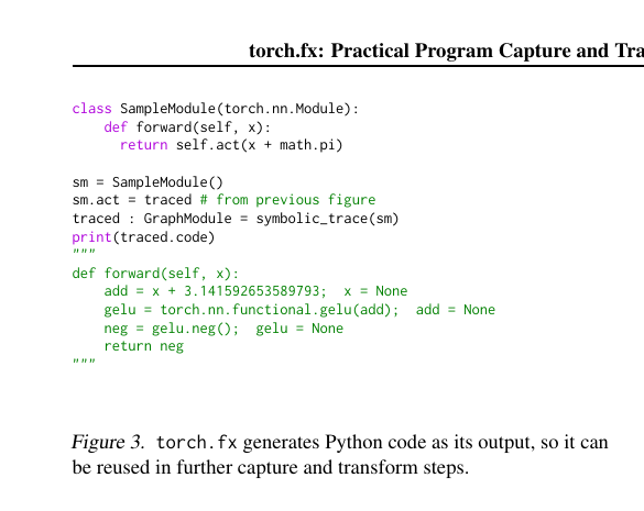
Figure 3 (Reed et al., 2022): torch.fx generates Python code as its output. Here the result of a previous relu→gelu replacement is installed as a sub-module and symbolically traced again — the constants (math.pi) are inlined and the full chain of transforms is visible in a single flat IR.
7. Design Decisions
7.1 No Control Flow in the IR
The most consequential design decision: torch.fx’s Graph has no if, while, or for nodes. This is not an oversight — it is central to the system’s simplicity.
Why control flow complicates transforms. With control flow in the IR, every analysis must be a fixpoint dataflow computation:
- Define a lattice of analysis values (e.g.
{unknown, dynamic, concrete_shape}). - Define a transfer function \(f_n\) for each node: given the analysis value of inputs, compute the analysis value of the output.
- Define a join \(\sqcup\) for merging values at control-flow merge points (e.g. after an
if). - Iterate until convergence.
For a basic block (no control flow), only the transfer function is needed — a single forward pass.
The paper gives shape analysis as a concrete example of the difference. For a basic block, shape propagation is \(O(n)\):
def propagate_shapes(graph: Graph, inputs: dict[str, tuple]):
    shapes = dict(inputs)
    for node in graph.nodes:
        if node.op == "placeholder":
            pass  # shape set from inputs
        elif node.op == "call_function":
            in_shapes = tuple(shapes[a.name] for a in node.args if isinstance(a, Node))
            # Transfer function for the specific op:
            shapes[node.name] = infer_shape(node.target, in_shapes)
    return shapes
With a loop in the IR, torch.cat in a loop body accumulates an unbounded shape — the analysis reaches a "dynamic" fixed point after arbitrarily many iterations. This “dynamic” value then poisons downstream analyses that need concrete shapes (e.g. ASIC memory planning).
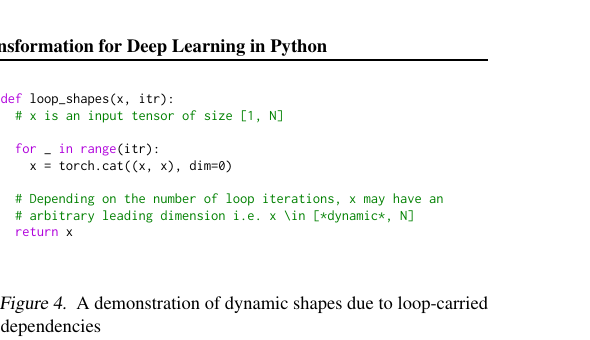
Figure 4 (Reed et al., 2022): A concrete illustration of loop-carried shape dynamics. After k iterations of torch.cat((x, x), dim=0), the leading dimension is \(2^k\) — not statically knowable. Shape analysis in a basic block IR avoids this entirely by simply not representing the loop.
If a traced function contains for i in range(n) where n is a Python constant (e.g. range(3)), the loop is unrolled by the tracer — it appears in the IR as 3 repetitions of the loop body. If n is data-dependent, the trace raises a TraceError.
7.2 Functional Graph, Stateful Modules
torch.fx’s Graph is functional — no node mutates another node’s output. But model parameters are state, and some operations have well-understood stateful semantics (e.g. BatchNorm tracks running mean/variance).
The solution: parameters and sub-modules live in GraphModule, outside the functional graph. The graph interacts with them via two opcodes:
- get_attr fetches a parameter by dotted path from the module hierarchy.
- call_module invokes a sub-module’s forward.
Transforms can modify both the graph (e.g. remove a BatchNorm node) and the module state (e.g. absorb the BN scale/shift into the preceding Conv weights) simultaneously, since they are co-located in the GraphModule.
# Both are accessible from a GraphModule:
gm: fx.GraphModule = fx.symbolic_trace(model)
gm.graph           # the functional Graph
gm.conv1           # the nn.Conv2d module (stateful parameters)
gm.conv1.weight    # the actual parameter tensor
7.3 AoT Capture Without Specialization
torch.fx traces ahead-of-time — once, at transform-authoring time, not on every inference call. The graph is not specialized to any particular input: no concrete shapes, dtypes, or scalar values flow through the symbolic trace (unless the Tracer is explicitly written to specialize).
This is in contrast to jit.trace (which specializes to example input shapes) and JIT systems like LazyTensor (which re-specialize on every call). The tradeoff:
| Property | torch.fx AoT | jit.trace AoT |
LazyTensor JIT |
|---|---|---|---|
| Handles data-dependent control flow | ❌ | ❌ | ✅ |
| Accidental shape specialization | ❌ | ✅ | ❌ |
| Re-capture overhead | ❌ | ❌ | ✅ |
| Observable failures | ✅ (TraceError) | ❌ (silent wrong output) | N/A |
Specialization is left to the transform. A quantization pass that needs to know tensor ranges can instrument the graph with observer nodes during a calibration phase — this is the transform deciding to specialize, not the capture mechanism.
8. Writing Graph Transforms
8.1 The Transform Pattern
All torch.fx transforms follow the same structure:
def my_transform(gm: fx.GraphModule) -> fx.GraphModule:
    graph = gm.graph
    for node in list(graph.nodes):  # iterate a copy — graph may be modified
        if <matches pattern>:
            with graph.inserting_after(node):
                new_node = graph.<create_node>(...)
            node.replace_all_uses_with(new_node)
            graph.erase_node(node)
    graph.lint()        # verify IR invariants (no dangling references, etc.)
    gm.recompile()      # regenerate forward() from the modified graph
    return gm
The graph mutation API:
- graph.inserting_after(node) / graph.inserting_before(node) — context managers that set the insertion point for subsequent node creation calls.
- node.replace_all_uses_with(new_node) — redirect all consumers of node to new_node.
- graph.erase_node(node) — remove node (only safe when it has no users).
- graph.lint() — check IR invariants: topological order, no dead references.
8.2 Activation Replacement
The paper’s Figure 2 shows the compact form of the activation replacement transform — fewer than 10 lines of Python for a complete graph rewrite pass:
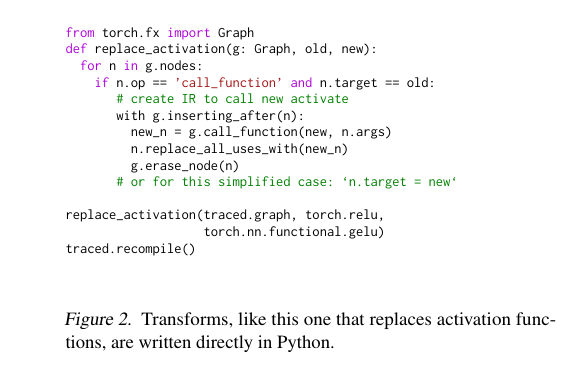
Figure 2 (Reed et al., 2022): The activation replacement transform from the paper. inserting_after sets the insertion point, replace_all_uses_with rewires all consumers, and erase_node removes the old node. The simplicity of this pass is a direct consequence of the Python-native IR.
The paper’s Figure 2 example — replacing all relu calls with gelu:
import torch
import torch.fx as fx
import torch.nn.functional as F

def replace_relu_with_gelu(gm: fx.GraphModule) -> fx.GraphModule:
    graph = gm.graph
    for node in list(graph.nodes):
        if node.op == "call_function" and node.target is torch.relu:
            with graph.inserting_after(node):
                gelu_node = graph.call_function(F.gelu, node.args, node.kwargs)
            node.replace_all_uses_with(gelu_node)
            graph.erase_node(node)
    graph.lint()
    gm.recompile()
    return gm


class SimpleNet(torch.nn.Module):
    def forward(self, x):
        return torch.relu(torch.relu(x) + 1.0)

gm = fx.symbolic_trace(SimpleNet())
print("Before:\n", gm.code)

replace_relu_with_gelu(gm)
print("After:\n", gm.code)

# Before:
#   relu   = torch.relu(x)
#   add    = relu + 1.0
#   relu_1 = torch.relu(add)
#   return relu_1
#
# After:
#   gelu   = torch.nn.functional.gelu(x)
#   add    = gelu + 1.0
#   gelu_1 = torch.nn.functional.gelu(add)
# return gelu_1call_method relu
This problem extends the activation replacement transform to cover method-style relu calls.
Prerequisites: 8.2 Activation Replacement, 5.1 The Six Opcodes
The replace_relu_with_gelu transform above only catches call_function nodes targeting torch.relu. However, users often write x.relu() (a call_method node with target "relu"). Extend the transform to also replace call_method relu nodes with call_function gelu nodes. Be precise about how args are structured differently for call_method vs. call_function.
Key insight: For a call_method node x.relu(), args[0] is the self tensor (the node for x). A call_function F.gelu(x) takes the same tensor as its first positional arg. The replacement is straightforward once you know the args convention.
Sketch:
for node in list(graph.nodes):
    if node.op == "call_function" and node.target is torch.relu:
        with graph.inserting_after(node):
            new = graph.call_function(F.gelu, node.args, node.kwargs)
        node.replace_all_uses_with(new)
        graph.erase_node(node)

    elif node.op == "call_method" and node.target == "relu":
        # args = (self_tensor, *positional_args) — here just (self_tensor,)
        self_tensor = node.args[0]
        with graph.inserting_after(node):
            new = graph.call_function(F.gelu, (self_tensor,), {})
        node.replace_all_uses_with(new)
        graph.erase_node(node)
Note: call_method nodes for relu should have no extra args beyond self, so node.args[0] is always the tensor.
8.3 Conv–BatchNorm Fusion
Conv–BN fusion is a canonical example of a transform that requires non-local program context (it must see two adjacent nodes) and must modify both the graph and the module state simultaneously.
The mathematical basis. A Conv2d followed by BatchNorm computes:
\[\text{BN}(\text{Conv}(x)) = \gamma \cdot \frac{W * x + b - \mu}{\sqrt{\sigma^2 + \epsilon}} + \beta\]
This is equivalent to a Conv2d with modified weight \(W'\) and bias \(b'\):
\[W' = \frac{\gamma}{\sqrt{\sigma^2 + \epsilon}} W, \qquad b' = \gamma \cdot \frac{b - \mu}{\sqrt{\sigma^2 + \epsilon}} + \beta\]
After folding, the BN node can be removed. The transform must:
1. Find every call_module → call_module pair where the first is a Conv2d and the second is a BatchNorm2d.
2. Compute \(W'\) and \(b'\) and write them into the Conv2d’s parameters.
3. Replace all uses of the BN node with the Conv node.
4. Erase the BN node.
def fuse_conv_bn(gm: fx.GraphModule) -> fx.GraphModule:
    graph = gm.graph
    for node in list(graph.nodes):
        # look for a BN node whose sole input is a Conv node
        if node.op != "call_module":
            continue
        bn = gm.get_submodule(node.target)
        if not isinstance(bn, torch.nn.BatchNorm2d) or not bn.track_running_stats:
            continue
        if len(node.args) != 1 or node.args[0].op != "call_module":
            continue
        conv_node = node.args[0]
        conv = gm.get_submodule(conv_node.target)
        if not isinstance(conv, torch.nn.Conv2d):
            continue

        # fold BN parameters into Conv weights
        with torch.no_grad():
            scale = bn.weight / (bn.running_var + bn.eps).sqrt()
            conv.weight.data *= scale[:, None, None, None]
            if conv.bias is None:
                conv.bias = torch.nn.Parameter(torch.zeros(conv.out_channels))
            conv.bias.data = (conv.bias.data - bn.running_mean) * scale + bn.bias

        # rewire graph: redirect BN's users to the Conv node
        node.replace_all_uses_with(conv_node)
        graph.erase_node(node)

    graph.lint()
    gm.recompile()
    return gm
The paper reports ~6% latency reduction on GPU and ~40% on CPU for ResNet50 with this transform.
8.4 Shape Propagation
torch.fx.passes.shape_prop.ShapeProp is a built-in interpreter pass that propagates shapes by executing the graph concretely with example inputs and recording the resulting tensor metadata on each node:
from torch.fx.passes.shape_prop import ShapeProp

model = torch.nn.Linear(8, 4)
gm = fx.symbolic_trace(model)

example = torch.randn(2, 8)
ShapeProp(gm).propagate(example)

for node in gm.graph.nodes:
    if "tensor_meta" in node.meta:
        print(node.name, node.meta["tensor_meta"].shape)

# x          torch.Size([2, 8])
# weight     torch.Size([4, 8])
# ...
# output     torch.Size([2, 4])
The underlying pattern — walking nodes in order and running each concretely — is a simple Interpreter:
class MiniInterpreter:
    """Run a Graph concretely to propagate metadata."""
    def __init__(self, gm: fx.GraphModule):
        self.gm = gm

    def run(self, *args):
        env: dict[str, Any] = {}
        arg_iter = iter(args)
        for node in self.gm.graph.nodes:
            if node.op == "placeholder":
                env[node.name] = next(arg_iter)
            elif node.op == "get_attr":
                env[node.name] = self.gm.get_parameter(node.target)
            elif node.op == "call_function":
                a = tuple(env[n.name] if isinstance(n, fx.Node) else n for n in node.args)
                env[node.name] = node.target(*a, **node.kwargs)
            elif node.op == "call_method":
                self_val = env[node.args[0].name]
                a = tuple(env[n.name] if isinstance(n, fx.Node) else n for n in node.args[1:])
                env[node.name] = getattr(self_val, node.target)(*a)
            elif node.op == "call_module":
                submod = self.gm.get_submodule(node.target)
                a = tuple(env[n.name] if isinstance(n, fx.Node) else n for n in node.args)
                env[node.name] = submod(*a)
            elif node.op == "output":
return env[node.args[0].name]This problem applies the Interpreter pattern to implement a FLOP counter.
Prerequisites: 8.4 Shape Propagation
Extend MiniInterpreter to count floating-point multiply-accumulate operations. For a call_function node targeting torch.mm(A, B) where \(A \in \mathbb{R}^{m \times k}\) and \(B \in \mathbb{R}^{k \times n}\), the FLOP count is \(2mkn\) (one multiply + one accumulate per entry). After running ShapeProp, tensor shapes are available in node.meta["tensor_meta"].shape. Sketch the implementation.
Key insight: After ShapeProp, each node’s meta["tensor_meta"] carries the output shape. For ops like mm, the input shapes determine the FLOP count. The interpreter can tally FLOPs without re-executing — just inspect node.meta.
Sketch:
def count_flops(gm: fx.GraphModule, example: torch.Tensor) -> int:
    ShapeProp(gm).propagate(example)  # populate node.meta with shapes
    total = 0
    for node in gm.graph.nodes:
        if node.op == "call_function" and node.target is torch.mm:
            # args[0].meta gives input A shape, args[1].meta gives B shape
            m, k = node.args[0].meta["tensor_meta"].shape
            k2, n = node.args[1].meta["tensor_meta"].shape
            assert k == k2
            total += 2 * m * k * n
        # extend for conv2d, linear, etc.
    return total
For torch.nn.functional.linear(x, w, b) where x ∈ R^{B×in}, w ∈ R^{out×in}: FLOPs = 2 * B * in * out (plus B * out for bias add).
9. Case Studies
The paper evaluates torch.fx across four application areas. The results establish that the simplicity of the IR pays off in implementation productivity as well as performance.
| Case Study | What torch.fx enabled | Key result |
|---|---|---|
| IR complexity | Simpler representation than TorchScript | 445 nodes for ResNet50 vs. 860 (jit.trace) vs. 2614 (jit.script) |
| Post-training quantization | Observer insertion + conversion in a single Python pass | 3.3× inference speedup on DeepRecommender (CPU, FBGEMM) |
| Conv–BN fusion | Non-local pattern match + simultaneous weight + graph modification | 6% GPU latency reduction, 40% CPU latency reduction on ResNet50 |
| Program scheduling | Hoist non-blocking RPC prefetch calls early in the graph | Up to 9% QPS improvement in large distributed training |
| TensorRT lowering | Translate FX graph to TensorRT IR + handle unsupported ops | 3.7× inference speedup on ResNet50 |
| Shape analysis | ShapeProp interpreter; symbolic shape propagation |
Foundation for quantization calibration and ASIC memory planning |
Figure 5 shows the concrete IR size difference for ResNet50. The TorchScript IR (left) requires explicit constant-construction nodes for every integer and list; the torch.fx IR (right) embeds them as immediate arguments, cutting node count by nearly 2×.
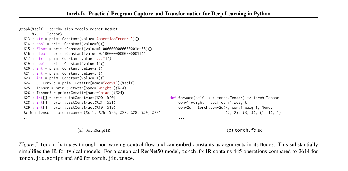
Figure 5 (Reed et al., 2022): TorchScript IR (left) vs. torch.fx IR (right) for the opening Conv2d of ResNet50. TorchScript emits separate prim::ListConstruct nodes for strides and padding; torch.fx embeds (2, 2) and (3, 3) directly as node arguments. For a full ResNet50, this reduces the IR from 860 nodes (jit.trace) or 2614 nodes (jit.script) down to 445 nodes.
The quantization result demonstrates the runtime benefit of operator-level reduction. Applying PTQ via torch.fx achieves up to 3.3× speedup across batch sizes on a server-class CPU:
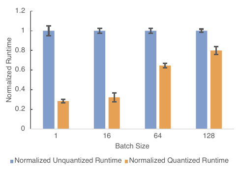
Figure 6 (Reed et al., 2022): Normalized inference runtime (lower is better) for torch.fx-based PTQ on DeepRecommender. Quantized runtime (orange) is 3–3.3× faster than FP32 (blue) at batch sizes 1, 16, and 64; the gap narrows at batch size 128 where memory bandwidth becomes less of a bottleneck.
The Conv–BN fusion transform achieves its largest relative gains on CPU where kernel launch overhead is proportionally greater:
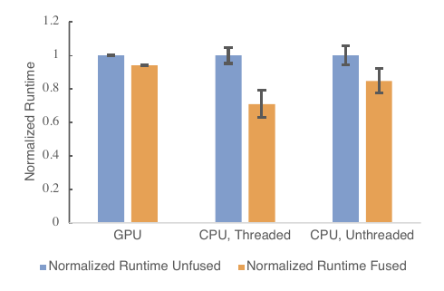
Figure 7 (Reed et al., 2022): Normalized inference runtime for torch.fx-based Conv–BN fusion on ResNet50. Fused (orange) vs. unfused (blue): ~6% speedup on GPU, ~30% on CPU threaded, ~15% on CPU unthreaded. The larger CPU gains reflect reduced memory bandwidth pressure from eliminating the BN read/write pass.
The TensorRT lowering pass delegates operator execution to a specialized inference engine, yielding the largest single-transform speedup:
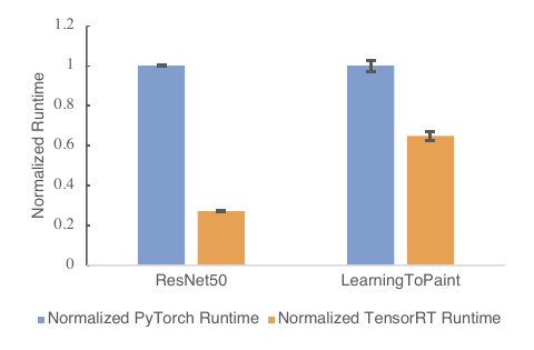
Figure 8 (Reed et al., 2022): Normalized inference runtime for torch.fx-based TensorRT lowering. TensorRT (orange) achieves 3.7× speedup on ResNet50 and ~1.6× on LearningToPaint vs. native PyTorch (blue). Unsupported operations fall back to eager PyTorch, explaining the smaller gain on the more heterogeneous LearningToPaint model.
The paper notes an order-of-magnitude productivity increase for quantization development compared to TorchScript, and fewer than 150 lines of Python for the full Conv-BN fusion transform including a test harness. This is the strongest argument for the torch.fx design philosophy: simpler IR = simpler transforms = faster development.
This problem sketches the preparation phase of post-training quantization using torch.fx.
Prerequisites: 8.1 The Transform Pattern, 9. Case Studies
Post-training quantization requires inserting “observer” modules after specific activation nodes (e.g. after every call_function targeting torch.relu). An observer records the min/max of the floating-point values flowing through it during calibration. Sketch a prepare_ptq transform that inserts observer modules after every relu call. What changes must be made to both the Graph and the GraphModule?
Key insight: Inserting an observer requires both (a) adding a call_module node to the graph (to call the observer during forward), and (b) registering the observer module on the GraphModule so the call_module node can find it by dotted path.
Sketch:
from torch.quantization import MinMaxObserver

def prepare_ptq(gm: fx.GraphModule) -> fx.GraphModule:
    graph = gm.graph
    observer_count = 0
    for node in list(graph.nodes):
        if node.op == "call_function" and node.target is torch.relu:
            # Register an observer module on the GraphModule
            obs_name = f"observer_{observer_count}"
            observer_count += 1
            gm.add_module(obs_name, MinMaxObserver())
            # Insert call_module node after the relu node
            with graph.inserting_after(node):
                obs_node = graph.call_module(obs_name, (node,))
            node.replace_all_uses_with(obs_node)
            # Restore: obs_node takes node as input (not itself)
            obs_node.args = (node,)
    graph.lint()
    gm.recompile()
    return gm
After prepare_ptq(gm), running calibration data through gm(x) automatically updates each observer’s min_val and max_val. The conversion phase then uses these statistics to choose quantization scales.
References
| Reference | Brief Summary | Link |
|---|---|---|
| Reed et al., “torch.fx: Practical Program Capture and Transformation for Deep Learning in Python” (MLSys 2022) | The primary source; 6-opcode IR, symbolic tracing, design decisions, case studies | arXiv 2112.08429 |
| PyTorch, “torch.fx Overview” (official docs) | API reference for Graph, Node, GraphModule, Tracer, Interpreter, Transformer |
docs.pytorch.org |
| PyTorch, “torch.fx: Symbolic Tracing” (tutorial) | Worked examples of symbolic tracing and graph transforms | docs.pytorch.org/tutorials |
| He, “Building a Conv/BN Fuser in FX” (tutorial) | Step-by-step implementation of the Conv–BN fusion transform | pytorch.org/tutorials |
| Ansel et al., “PyTorch 2: Faster ML Through Dynamic Bytecode Transformation” (ASPLOS 2024) | How torch.fx becomes the IR that TorchDynamo, AOTAutograd, and TorchInductor pass between stages | arXiv 2304.01277 |
| Yang, “PyTorch Internals” (blog, 2019) | Background on the dispatcher and tensor model that torch.fx sits on top of | blog.ezyang.com |