Rejection Sampling as Reinforcement Learning
Anchored to: Zeng et al. (2025), A Minimalist Approach to LLM Reasoning
Table of Contents
- 1. The RL Framework for LLM Post-Training
- 2. Classical Rejection Sampling
- 3. Rejection Sampling for LLMs: RAFT
- 4. The Distribution Shift Problem and RAFT++
- 5. Entropy Collapse
- 6. Policy Gradient Methods
- 7. Reinforce-Rej: Bridging the Gap
- 8. Summary Comparison
- References
1. The RL Framework for LLM Post-Training 🎯
After supervised pre-training, a language model \(\pi_\text{ref}\) has learned to predict text but not to optimize for a specific goal — e.g., solving math problems correctly or following human instructions. Reinforcement learning provides the framework for this second stage.
The setup: - State: the prompt \(x\) (e.g., a math problem) - Action: a generated response \(y = (a_1, a_2, \ldots, a_T)\) (a sequence of tokens) - Reward: a scalar \(r(x, y)\) evaluating the quality of the response (e.g., 1 if correct, 0 if not) - Policy: \(\pi_\theta(y|x)\), the language model parameterized by \(\theta\)
Unlike classical RL with short action sequences, the “action” here is an entire token sequence — the credit assignment problem is therefore collapsed: the reward arrives only at the end of the full generation.
1.1 The KL-Regularized Objective
A naive objective \(\max_\theta \mathbb{E}_{y \sim \pi_\theta}[r(x,y)]\) is unstable: the model can exploit the reward function by drifting arbitrarily far from \(\pi_\text{ref}\), producing degenerate outputs that score well but are incoherent (reward hacking).
The standard fix is to add a KL regularization penalty:
\[\mathcal{J}(\theta) = \mathbb{E}_{x \sim \mathcal{D}}\left[\mathbb{E}_{y \sim \pi_\theta(\cdot|x)}\left[r(x,y)\right] - \beta \cdot D_\text{KL}\!\left(\pi_\theta(\cdot|x) \,\|\, \pi_\text{ref}(\cdot|x)\right)\right]\]
where \(\beta > 0\) is a temperature that controls the strength of the regularization. The KL term penalizes the policy for deviating from the reference model, which:
- Prevents reward hacking
- Preserves the language modeling prior (fluency, coherence)
- Keeps the optimization well-conditioned
1.2 The Closed-Form Optimal Policy
The KL-regularized objective is a strictly concave functional over the policy distribution — it has a unique global maximizer. We find it via the calculus of variations.
Setting up the problem. Fixing \(x\), define the functional over distributions on \(y\):
\[\mathcal{J}[\pi] = \sum_y \pi(y|x)\,r(x,y) - \beta \sum_y \pi(y|x)\log\frac{\pi(y|x)}{\pi_\text{ref}(y|x)}\]
subject to \(\sum_y \pi(y|x) = 1\). We want \(\frac{\delta \mathcal{J}}{\delta \pi(y)} = 0\) for all \(y\).
Functional derivative. In the discrete case, \(\frac{\delta \mathcal{J}}{\delta \pi(y)} = \frac{\partial \mathcal{J}}{\partial \pi(y)}\) — an ordinary partial derivative, treating each \(\pi(y|x)\) as an independent variable. In the continuous case this is the Gateaux derivative, defined by the identity
\[\frac{d}{d\epsilon}\mathcal{J}[\pi + \epsilon\eta]\bigg|_{\epsilon=0} = \sum_y \frac{\delta \mathcal{J}}{\delta \pi(y)}\,\eta(y) \quad \text{for all test functions } \eta\]
The discrete and continuous cases are formally identical; we work with the discrete form.
Computing term by term:
\[\frac{\partial}{\partial \pi(y)}\sum_{y'}\pi(y')\,r(x,y') = r(x,y)\]
\[\frac{\partial}{\partial \pi(y)}\sum_{y'}\pi(y')\log\frac{\pi(y')}{\pi_\text{ref}(y')} = \log\frac{\pi(y)}{\pi_\text{ref}(y)} + 1 \qquad \left(\frac{d}{dp}[p\log p] = \log p + 1\right)\]
Lagrangian and stationarity. Introduce \(\lambda\) to enforce normalization:
\[\mathcal{L}[\pi,\lambda] = \mathcal{J}[\pi] - \lambda\!\left(\sum_y \pi(y|x) - 1\right)\]
Setting \(\frac{\partial \mathcal{L}}{\partial \pi(y)} = 0\) for all \(y\):
\[r(x,y) - \beta\!\left(\log\frac{\pi(y)}{\pi_\text{ref}(y)} + 1\right) - \lambda = 0\]
Solving for \(\pi(y)\):
\[\log\frac{\pi(y)}{\pi_\text{ref}(y)} = \frac{r(x,y)}{\beta} - 1 - \frac{\lambda}{\beta}\]
\[\pi(y|x) = \pi_\text{ref}(y|x)\,\exp\!\left(\frac{r(x,y)}{\beta}\right)\cdot\underbrace{e^{-1 - \lambda/\beta}}_{\text{constant in }y}\]
Fixing the constant. The normalization \(\sum_y \pi(y|x) = 1\) determines \(\lambda\):
\[e^{-1-\lambda/\beta} = \frac{1}{\displaystyle\sum_{y'}\pi_\text{ref}(y'|x)\,e^{r(x,y')/\beta}} \equiv \frac{1}{Z(x)}\]
Substituting back gives the closed-form optimal policy:
\[\boxed{\pi^*(y|x) = \frac{\pi_\text{ref}(y|x)\,e^{r(x,y)/\beta}}{Z(x)}}\]
Why this is a maximum, not a saddle point. The reward term \(\sum_y \pi(y) r(x,y)\) is linear in \(\pi\) (both convex and concave). The KL term \(D_\text{KL}(\pi\|\pi_\text{ref}) = \sum_y \pi\log(\pi/\pi_\text{ref})\) is strictly convex in \(\pi\) (since \(p \mapsto p\log p\) is strictly convex). Therefore \(-\beta D_\text{KL}\) is strictly concave, making \(\mathcal{J}\) strictly concave overall — the stationarity condition is both necessary and sufficient for a unique global maximum.
Key result: \(\pi^*\) is a Gibbs distribution (Boltzmann distribution) over responses, where the reference model provides the base measure and the reward acts as an energy function. Higher reward → exponentially higher probability under \(\pi^*\).
- \(\beta \to \infty\): the KL penalty dominates, so \(\pi^* \approx \pi_\text{ref}\) — no learning happens. - \(\beta \to 0\): the reward dominates, so \(\pi^*\) concentrates all mass on the highest-reward response — mode collapse. - Intermediate \(\beta\): balances exploration (staying broad like \(\pi_\text{ref}\)) with exploitation (concentrating on high-reward regions).
\(Z(x) = \sum_y \pi_\text{ref}(y|x)\,e^{r(x,y)/\beta}\) sums over all possible token sequences — exponentially many. This is the same object that makes inference in energy-based models hard, and the same one DPO sidesteps by working in ratios \(\pi^*(y|x)/\pi^*(y'|x)\) where \(Z(x)\) cancels. Every practical post-training algorithm is a strategy for optimizing toward \(\pi^*\) without computing \(Z(x)\).
This problem shows that even without computing \(Z(x)\), its structure constrains the optimal policy.
Prerequisites: §1.2 The Closed-Form Optimal Policy
For binary reward \(r \in \{0,1\}\), let \(p_\text{ref}(x) = \sum_{y:r=1}\pi_\text{ref}(y|x)\) be the reference model’s success probability. Show that \(Z(x) \geq e^{1/\beta}\,p_\text{ref}(x)\), and conclude that \(\pi^*(y|x) \leq \pi_\text{ref}(y|x)/p_\text{ref}(x)\) for any correct response \(y\).
Key insight: \(Z(x) = \sum_{y:r=1}\pi_\text{ref}(y|x)e^{1/\beta} + \sum_{y:r=0}\pi_\text{ref}(y|x) \geq e^{1/\beta} p_\text{ref}(x)\).
Sketch: For correct \(y\): \(\pi^*(y|x) = \pi_\text{ref}(y|x) e^{1/\beta}/Z(x) \leq \pi_\text{ref}(y|x) e^{1/\beta}/(e^{1/\beta} p_\text{ref}(x)) = \pi_\text{ref}(y|x)/p_\text{ref}(x)\). The optimal policy redistributes mass from incorrect to correct responses, bounded above by \(\pi_\text{ref}\) renormalized to the correct-answer set.
2. Classical Rejection Sampling 🎲
Rejection sampling is a fundamental Monte Carlo technique for drawing exact samples from a target distribution \(p^*(y)\) that is hard to sample from directly, using a proposal distribution \(q(y)\) that is easy to sample from. Critically, it requires only the ability to evaluate the unnormalized density \(\tilde{p}(y) \propto p^*(y)\) — it does not require computing the normalizing constant \(Z\).
2.1 The Algorithm
Given: - A target \(p^*(y) = \tilde{p}(y)/Z\), where \(\tilde{p}\) is the unnormalized density and \(Z\) is unknown - A proposal \(q(y)\) that is easy to sample from - A constant \(M\) such that \(\tilde{p}(y) \leq M \cdot q(y)\) for all \(y\)
Repeat until acceptance: 1. Sample \(y \sim q(y)\) 2. Sample \(u \sim \text{Uniform}[0, 1]\) 3. Accept \(y\) if \(u \leq \dfrac{\tilde{p}(y)}{M \cdot q(y)}\); otherwise reject and go to step 1
The collection of accepted samples is exactly i.i.d. from \(p^*\).
2.2 Correctness
Claim: The marginal distribution of an accepted sample is \(p^*\).
Proof. The joint law of \((y, u)\) before the acceptance test is \(q(y) \cdot \mathbf{1}[u \in [0,1]]\). A pair \((y, u)\) is accepted iff \(u \leq \tilde{p}(y)/(Mq(y))\). The marginal density over accepted \(y\) is:
\[p(y \mid \text{accept}) \propto q(y) \cdot \Pr\!\left(u \leq \frac{\tilde{p}(y)}{Mq(y)}\right) = q(y) \cdot \frac{\tilde{p}(y)}{Mq(y)} = \frac{\tilde{p}(y)}{M}\]
Normalizing: \(p(y \mid \text{accept}) = \tilde{p}(y)/Z = p^*(y)\). \(\square\)
The acceptance region in \((y, u)\) space is the region under the curve \(u = \tilde{p}(y)/(Mq(y))\). Uniform sampling in the rectangle \([0,1] \times \text{support}(q)\) and keeping only points in this region is equivalent to sampling uniformly under the graph of \(\tilde{p}/M\) — which gives \(\tilde{p}\) as the marginal. This is the graphical interpretation of rejection sampling.
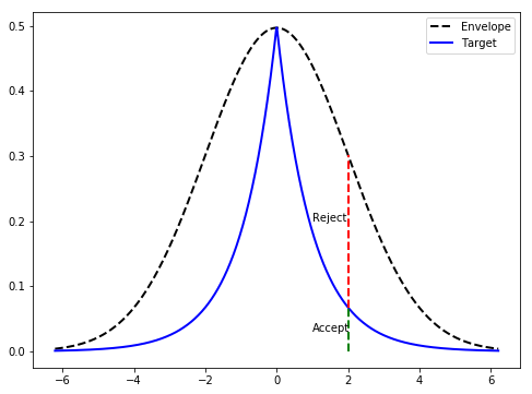
Figure 1 (Guzman, 2018): The dashed envelope \(M \cdot q(y)\) dominates the solid target \(\tilde{p}(y)\) everywhere. At a proposed sample near \(y=2\), the red segment (above \(\tilde{p}\), inside the envelope) causes rejection; the green segment (below \(\tilde{p}\)) would cause acceptance. The ratio of green to total column height equals the acceptance probability \(\tilde{p}(y)/(Mq(y))\).
2.3 Efficiency and the Optimal Bound
The overall probability of acceptance on any single proposal is:
\[\Pr(\text{accept}) = \int q(y)\,\frac{\tilde{p}(y)}{Mq(y)}\,dy = \frac{1}{M}\int \tilde{p}(y)\,dy = \frac{Z}{M}\]
To maximize efficiency, take the tightest upper bound:
\[M^* = \sup_y \frac{\tilde{p}(y)}{q(y)}\]
giving maximum acceptance rate \(Z/M^*\). The expected number of proposals per accepted sample is \(M^*/Z\).
In high dimensions, rejection sampling becomes catastrophically inefficient. When \(p^*\) concentrates on a low-measure subset of \(q\)’s support, \(M^*\) is large and \(Z/M^* \approx 0\). For LLMs the space of token sequences is astronomically large — naive rejection sampling from \(\pi_\text{ref}\) would accept almost nothing on hard problems. This motivates running multiple proposals per prompt and imitation-learning from the accepted ones rather than sampling one at a time.
2.4 Connection to the Optimal LLM Policy
Set proposal \(q = \pi_\text{ref}\) and target \(p^* = \pi^*(y|x)\). The unnormalized density is:
\[\tilde{p}(y) = \pi_\text{ref}(y|x)\,e^{r(x,y)/\beta}\]
The acceptance probability becomes:
\[\Pr(\text{accept}\;y) = \frac{\tilde{p}(y)}{M \cdot \pi_\text{ref}(y|x)} = \frac{e^{r(x,y)/\beta}}{M}\]
with tightest bound \(M^* = e^{r_\text{max}/\beta}\).
For binary reward and \(\beta \to \infty\): Both correct and incorrect responses have \(e^{r/\beta} \to 1\) (since \(e^{0/\beta} = e^{1/\beta} \to 1\)), but their ratio diverges — the acceptance criterion collapses to \(\mathbf{1}[r(x,y)=1]\). Accept iff the response is correct. This is precisely the RAFT filter step, with \(\pi_\text{ref}\) replaced by the current policy \(\pi_\theta\).
2.5 Relationship to Importance Sampling
Both rejection sampling and importance sampling (IS) solve the same problem — computing expectations or drawing samples under a target \(p^*\) using a tractable proposal \(q\) — and both are built from the same primitive: the importance weight
\[w(y) = \frac{p^*(y)}{q(y)} = \frac{\tilde{p}(y)}{Z \cdot q(y)}\]
The two methods differ only in how they use \(w\).
Importance sampling keeps every proposal but reweights it:
\[\mathbb{E}_{p^*}[f(y)] = \mathbb{E}_q\!\left[f(y)\,w(y)\right] \approx \frac{1}{n}\sum_{i=1}^n f(y_i)\,w(y_i), \quad y_i \sim q\]
When \(Z\) is unknown (as with \(\pi^*\) for LLMs), the self-normalized estimator is used:
\[\hat{\mu}_\text{SNIS} = \frac{\sum_i f(y_i)\,\tilde{w}_i}{\sum_i \tilde{w}_i}, \quad \tilde{w}_i = \frac{\tilde{p}(y_i)}{q(y_i)}\]
This is consistent but biased for finite \(n\).
Rejection sampling binarizes the same weight: a proposal \(y \sim q\) is accepted iff \(u \leq \tilde{p}(y)/(Mq(y)) = w(y)/(M/Z)\). The effective weight assigned to each proposal is therefore
\[w_\text{RS}(y_i) = \begin{cases} 1 & \text{accepted (high } w_i\text{)} \\ 0 & \text{rejected (low } w_i\text{)} \end{cases}\]
RS achieves exact, equal-weight samples from \(p^*\) by paying a cost in wasted proposals. IS retains all proposals by paying a cost in weight variance. The trade-off is summarized:
| Importance Sampling | Rejection Sampling | |
|---|---|---|
| Proposals kept | All (reweighted) | Only accepted |
| Weight per sample | Continuous \(\tilde{w}_i\) | Binary \(\{0,1\}\) |
| Output | Weighted approximation to \(p^*\) | Exact i.i.d. samples from \(p^*\) |
| Failure mode | High weight variance | Low acceptance rate |
Both failure modes have the same root cause. When \(p^*\) and \(q\) are poorly matched, importance weights are highly variable — a few proposals \(y\) with large \(w(y)\) dominate. This is equivalent to a low RS acceptance rate (most proposals fall in the low-\(w\) region and are rejected). Quantitatively, the IS estimator variance and the RS acceptance rate are controlled by the same quantity:
\[\text{Var}_q[w(y)] = \mathbb{E}_q[w^2] - 1 = \frac{M^*}{Z} - 1 = \frac{1}{\text{acceptance rate}} - 1\]
so high IS variance ↔︎ low acceptance rate. Mismatch between \(p^*\) and \(q\) hurts both methods equally.
Both IS and RS produce a weighted sample set \(\{(y_i, w_i)\}\) approximating \(p^*\). IS uses continuous weights; RS binarizes them at a threshold. The general framework of weighted Monte Carlo — keep all proposals, assign weights, normalize — subsumes IS as the \(M \to \infty\) limit (never reject anything) and RS as the special case where weights are thresholded to \(\{0,1\}\).
The RAFT / RAFT++ reread. This dichotomy maps exactly onto the two algorithms:
- RAFT implements RS: draw \(y_i \sim \pi_\theta\), assign binary weights (accept iff \(r=1\)), imitate accepted samples via SFT.
- RAFT++ implements an IS correction on top: the per-token ratio \(s_t = \pi_\theta/\pi_{\theta_\text{old}}\) reweights samples collected under the old policy to produce an unbiased estimate under the current policy — this is self-normalized IS correcting for the off-policy gap. The PPO clip \(s_t \in [1-\epsilon, 1+\epsilon]\) plays the role of the envelope \(M\), bounding the weight ratio to prevent any single sample from dominating.
This problem connects rejection sampling efficiency to the “best-of-n” inference-time scaling strategy.
Prerequisites: §2.3 Efficiency and the Optimal Bound, §2.4 Connection to the Optimal LLM Policy
Suppose \(\pi_\text{ref}\) solves a given problem with probability \(p\). You generate \(n\) independent samples and accept the first correct one (best-of-\(n\)). (a) What is the probability that at least one sample is accepted? (b) How many samples do you need in expectation to get one accepted? (c) As \(p \to 0\), how does this scale, and what does it imply about RAFT on hard problems?
Key insight: Each sample is accepted independently with probability \(p\), so the count of accepted samples is \(\text{Binomial}(n, p)\).
Sketch: (a) \(\Pr(\text{at least one}) = 1 - (1-p)^n \approx 1 - e^{-np}\) for small \(p\). (b) Expected proposals until first acceptance \(= 1/p\) (geometric). To have a \(1-\delta\) chance of at least one, need \(n \gtrsim \log(1/\delta)/p\). (c) As \(p \to 0\), need \(n \sim 1/p\) proposals — which grows without bound. For RAFT, this means the accepted set \(\mathcal{D}_+\) becomes sparse on hard problems, starving the model of training signal and causing performance to plateau before hard problems are solved.
3. Rejection Sampling for LLMs: RAFT 🤖
RAFT (Reward-rAnked Fine-Tuning) is the simplest possible algorithm for post-training: generate candidates, keep the good ones, imitate them.
3.1 The Algorithm
For each prompt \(x\) in the training set:
- Sample \(n\) responses \(y_1, \ldots, y_n \sim \pi_\theta(\cdot|x)\) from the current policy
- Filter to the accepted set \(\mathcal{D}_+ = \{(x, y_i) : r(x, y_i) = 1\}\) (correct answers only)
- Fine-tune on \(\mathcal{D}_+\) via maximum likelihood:
\[\mathcal{L}^\text{RAFT}(\theta) = -\sum_{(x,y) \in \mathcal{D}_+} \log \pi_\theta(y|x)\]
This is just supervised fine-tuning (SFT) on filtered data.
3.2 Why This Is RL
At first glance, RAFT looks like supervised learning — it is just SFT on some data. But the data is generated and filtered by a reward signal, which makes it RL in a deep sense.
📐 The formal connection: Sampling \(y \sim \pi_\theta\) and accepting iff \(r(x,y)=1\) defines a distribution over accepted samples:
\[q(y|x) \propto \pi_\theta(y|x) \cdot \mathbf{1}[r(x,y)=1]\]
This is the binary-reward, \(\beta \to \infty\) limit of the optimal policy \(\pi^*\) with \(\pi_\text{ref}\) replaced by \(\pi_\theta\). The accepted sample distribution approximates \(\pi^*\), and RAFT trains \(\pi_\theta\) to imitate it via SFT.
3.3 The Imitation Learning Interpretation
RAFT can be read as behavioral cloning from an improved demonstrator:
- Run the current policy \(\pi_\theta\) to collect rollouts
- Filter rollouts using the reward as a success criterion
- Imitate the successful rollouts with SFT
The contrast with policy gradient methods:
| RAFT | REINFORCE | |
|---|---|---|
| Uses negative samples? | ❌ | ✅ |
| Gradient through reward? | ❌ | ✅ |
| Loss type | SFT (MLE) | Policy gradient |
| Credit assignment | Implicit (filter) | Explicit (gradient) |
This problem establishes the formal equivalence between RAFT and distribution matching to \(\pi^*\).
Prerequisites: §1.2 The Closed-Form Optimal Policy, §3.1 The Algorithm
Show that the RAFT loss \(\mathcal{L}^\text{RAFT}(\theta) = -\mathbb{E}_{(x,y) \sim \mathcal{D}_+}[\log \pi_\theta(y|x)]\) is equivalent (up to a constant) to minimizing \(D_\text{KL}(\hat{\pi}^* \| \pi_\theta)\), where \(\hat{\pi}^*\) is the empirical distribution over accepted samples. What does this imply about what RAFT is “trying” to do?
Key insight: \(D_\text{KL}(\hat\pi^* \| \pi_\theta) = \sum_{(x,y) \in \mathcal{D}_+} \hat\pi^*(y|x)\log\hat\pi^*(y|x) - \hat\pi^*(y|x)\log\pi_\theta(y|x)\). The first term is the entropy of \(\hat\pi^*\) — constant w.r.t. \(\theta\). Minimizing KL is therefore equivalent to maximizing \(\sum \hat\pi^* \log \pi_\theta\), which (with uniform weights over \(\mathcal{D}_+\)) is exactly \(-\mathcal{L}^\text{RAFT}\).
Sketch: RAFT is doing maximum likelihood estimation of \(\pi^*\) — fitting \(\pi_\theta\) to match the accepted sample distribution (a Monte Carlo approximation of \(\pi^*\)). This is RL via distribution matching, not via explicit gradient signals.
4. The Distribution Shift Problem and RAFT++ ⚠️
4.1 Why Shift Happens
RAFT has a subtle flaw: the accepted samples \(\mathcal{D}_+\) are collected from policy \(\pi_{\theta_\text{old}}\), but after each gradient update, \(\pi_\theta\) changes. If a replay buffer is used (reusing old data), the data distribution no longer matches the current policy.
This is the off-policy problem. The loss being minimized is:
\[\mathbb{E}_{y \sim \pi_{\theta_\text{old}}(\cdot|x),\, r(x,y)=1}[\log \pi_\theta(y|x)]\]
but the policy being updated is \(\pi_\theta \neq \pi_{\theta_\text{old}}\). The gradient is a biased estimator of the on-policy gradient.
4.2 Importance Sampling Correction
RAFT++ corrects for this bias. Define the per-token importance ratio:
\[s_t(\theta) = \frac{\pi_\theta(a_t | x, a_{1:t-1})}{\pi_{\theta_\text{old}}(a_t | x, a_{1:t-1})}\]
The corrected loss clips the ratio to \([1-\epsilon, 1+\epsilon]\) (PPO-style) to prevent large updates:
\[\mathcal{L}^\text{RAFT++}(\theta) = \frac{1}{|\mathcal{D}|}\sum_{(x,a) \in \mathcal{D}}\frac{1}{|a|}\sum_{t=1}^{|a|}\min\!\left(s_t(\theta),\, \text{clip}(s_t(\theta), 1{-}\epsilon, 1{+}\epsilon)\right) \cdot \mathbf{1}[r(x,a) = 1]\]
The identity \(\mathbb{E}_{y \sim \pi_\text{old}}[f(y)] = \mathbb{E}_{y \sim \pi}\!\left[f(y) \cdot \frac{\pi_\text{old}(y)}{\pi(y)}\right]\) is reversible: reweighting old samples by \(\pi_\theta/\pi_{\theta_\text{old}}\) gives an unbiased estimate of the on-policy expectation.
RAFT++ is essentially PPO restricted to positive samples. The clipping prevents the policy from moving too far from where the data was collected, stabilizing training.
5. Entropy Collapse 📉
A critical failure mode of RAFT (and to a lesser degree RAFT++) is entropy collapse: the output distribution rapidly narrows, concentrating mass on a small set of known-good responses.
Formally, the policy entropy is:
\[\mathcal{H}(\pi_\theta(\cdot|x)) = -\sum_y \pi_\theta(y|x)\log\pi_\theta(y|x)\]
RAFT only applies positive gradient (increasing \(\pi_\theta(y|x)\) for \(y\) with \(r=1\)) with no corresponding negative gradient (decreasing probability of \(r=0\) responses explicitly). The normalization constraint \(\sum_y \pi_\theta(y|x) = 1\) means accepted responses gaining mass implicitly forces others to lose mass — but this implicit decrease is uncontrolled and non-specific, failing to target genuinely bad responses.
The consequence: - Early in training: broad exploration, many diverse solutions discovered - As training continues: policy concentrates on a few known-good patterns - Entropy falls sharply → exploration ceases → performance plateaus
High entropy is not a goal in itself — you want the policy to concentrate on correct answers. But premature collapse means the model stops exploring and gets stuck at a local optimum. Entropy collapse in RAFT happens before the policy has found high-quality diverse solutions.
This problem builds intuition for why positive-only updates collapse entropy.
Prerequisites: §5 Entropy Collapse
Consider a toy setting: binary output space \(\{0, 1\}\) with reward \(r(1)=1\), \(r(0)=0\), and policy \(\pi_\theta(1|x) = p\). The RAFT update maximizes \(\log p\). Show that the entropy \(\mathcal{H}(p) = -p\log p - (1-p)\log(1-p)\) is monotonically decreasing once \(p > 0.5\). What does this say about the long-run behavior of RAFT?
Key insight: \(\frac{d\mathcal{H}}{dp} = \log\frac{1-p}{p}\). This is negative iff \(p > 0.5\). The RAFT gradient always increases \(p\) toward 1, so once \(p > 0.5\), entropy monotonically decreases toward 0.
Sketch: In the limit \(p \to 1\), \(\mathcal{H} \to 0\) — the policy becomes deterministic. In a multi-dimensional setting with many possible responses, the same logic applies: positive-only training drives the distribution toward a near-deterministic peak on learned patterns, terminating exploration.
6. Policy Gradient Methods 📐
6.1 REINFORCE
The policy gradient theorem gives a tractable estimator of \(\nabla_\theta \mathcal{J}\):
\[\nabla_\theta \mathcal{J}(\theta) = \mathbb{E}_{x \sim \mathcal{D}}\left[\mathbb{E}_{y \sim \pi_\theta(\cdot|x)}\left[\nabla_\theta \log \pi_\theta(y|x) \cdot r(x,y)\right]\right]\]
The key identity is \(\nabla_\theta \mathbb{E}_{y \sim \pi_\theta}[r] = \mathbb{E}[\nabla_\theta \log \pi_\theta \cdot r]\) — the log-derivative trick, which allows gradient computation without differentiating through the sampling process. With PPO-style clipping for stability:
\[\mathcal{L}^\text{REINFORCE}(\theta) = \frac{1}{|\mathcal{D}|}\sum_{(x,a) \in \mathcal{D}}\frac{1}{|a|}\sum_{t=1}^{|a|}\min\!\left(s_t(\theta),\, \text{clip}(s_t(\theta), 1{-}\epsilon, 1{+}\epsilon)\right) \cdot r(x,a)\]
With binary reward and no baseline, zero-reward responses produce zero gradient — not a negative gradient. The repulsive signal requires a baseline:
With baseline \(b\), the gradient uses advantage \(r(x,y) - b\) instead of raw reward. For prompts where all responses are incorrect, the advantage is \(0 - b < 0\) — a genuine push away from those responses. This is the mechanism by which negative samples aid learning.
6.2 GRPO: Group Relative Policy Optimization
GRPO samples \(n\) responses per prompt and computes a within-group normalized advantage:
\[A(x, y_i) = \frac{r_i - \mu_r}{\sigma_r}, \quad \mu_r = \frac{1}{n}\sum_{j=1}^n r_j, \quad \sigma_r = \sqrt{\frac{1}{n}\sum_{j=1}^n (r_j - \mu_r)^2}\]
This normalization has two effects: 1. Centering: correct responses in a mostly-correct group get low positive advantage; correct responses in a mostly-incorrect group get high positive advantage 2. Scaling: gradient magnitude is standardized across prompts with very different success rates
Surprisingly, the paper shows reward normalization contributes minimally to GRPO’s empirical gains over REINFORCE. The dominant benefit is the use of negative samples via the advantage.
6.3 The Role of Negative Samples
The paper makes a nuanced distinction:
| Prompt type | Effect of including |
|---|---|
| Mixed (some correct, some not) | ✅ Helpful — repulsive gradient on incorrect responses |
| All-incorrect | ❌ Harmful — high-variance gradient with no positive signal |
| All-correct | ❌ Harmful — trivially high reward, no discriminative signal |
Filtering all-incorrect prompts is what actually drives GRPO’s gains over naive REINFORCE. This is the key insight of Reinforce-Rej.
7. Reinforce-Rej: Bridging the Gap 🔑
Reinforce-Rej is the paper’s proposed algorithm: run REINFORCE with clipping, but filter to prompts with mixed outcomes:
\[\mathcal{D}^\text{Rej} = \left\{(x, \{y_i\}) : 0 < \sum_i r_i < n\right\}\]
This keeps only informative prompts and trains REINFORCE on them with normalized advantages.
The result: comparable performance to GRPO with: - Better KL efficiency (same reward with less divergence from \(\pi_\text{ref}\)) - Better entropy stability than RAFT (no collapse) - Simpler implementation than full GRPO
When all \(n\) samples fail (\(r_i = 0\)), advantage normalization gives \(A_i = (0-0)/0\) — undefined or numerically zero after smoothing. These prompts contribute gradient noise with no positive learning signal, destabilizing training.
8. Summary Comparison 📊
| Algorithm | Uses negatives | Distribution shift | Entropy stability | Complexity |
|---|---|---|---|---|
| RAFT | ❌ | Ignored | Poor (collapses) | Very low |
| RAFT++ | ❌ | Importance sampling | Moderate | Low |
| REINFORCE | ✅ | Importance sampling | Good | Moderate |
| GRPO | ✅ | Importance sampling | Good | Moderate |
| Reinforce-Rej | ✅ (filtered) | Importance sampling | Good | Low |
The big picture: The gap between RAFT and GRPO is not about algorithmic sophistication — it is about whether negative samples provide a repulsive gradient. Reinforce-Rej shows this gap can be closed with a simple filter.
References
| Reference Name | Brief Summary | Link |
|---|---|---|
| Zeng et al. (2025), A Minimalist Approach to LLM Reasoning | Compares RAFT, RAFT++, REINFORCE, GRPO for math reasoning; introduces Reinforce-Rej; identifies entropy collapse and negative-sample filtering as key factors | arXiv:2504.11343 |
| Dong et al. (2023), RAFT: Reward rAnked FineTuning | Original RAFT paper proposing rejection-sampling-based fine-tuning for alignment | arXiv:2304.06767 |
| Shao et al. (2024), DeepSeekMath | Introduces GRPO (Group Relative Policy Optimization) for mathematical reasoning | arXiv:2402.03300 |
| Ziegler et al. (2019), Fine-Tuning Language Models from Human Preferences | Foundational RLHF paper establishing the KL-regularized RL objective for LLMs | arXiv:1909.08593 |
| Rafailov et al. (2023), Direct Preference Optimization | Shows the optimal KL-regularized policy is a Gibbs distribution; derives DPO from this by working in ratios to cancel \(Z(x)\) | arXiv:2305.18290 |
| Williams (1992), Simple Statistical Gradient-Following Algorithms | Original REINFORCE algorithm; establishes the log-derivative trick for policy gradient estimation | Machine Learning 8(3-4) |
| Von Neumann (1951), Various techniques used in connection with random digits | Original rejection sampling algorithm | NBS Applied Mathematics Series |