Generative Recommender with End-to-End Learnable Item Tokenization
Enze Liu, Bowen Zheng, Cheng Ling, Lantao Hu, Han Li, Wayne Xin Zhao — Renmin University of China & Kuaishou Inc. ArXiv 2409.05546, 2024.
| Dimension | Prior State | This Paper | Key Result |
|---|---|---|---|
| Tokenizer–recommender coupling | RQ-VAE trained separately on reconstruction objective; codes fixed during recommendation training | Alternating optimization mutually refines tokenizer and recommender | w/o alternating training: −17.6% Recall@5 on Instruments |
| Recommendation signal in codes | Codes optimize reconstruction fidelity of content embeddings | SIA + PSA alignment objectives inject recommendation signal into codebook learning | Ablating both alignments: −3.9% Recall@5, −3.6% NDCG@5 (Instruments) |
| Encoder–item alignment | No explicit alignment between encoder hidden states and the item’s token distribution | SIA minimizes symmetric KL between encoder output and item’s codebook distributions | Ablating SIA alone: −0.5% Recall@5 |
| Decoder–item alignment | No alignment between decoded user preference vector and item embedding | PSA aligns first decoder hidden state with reconstructed item embedding via InfoNCE | Ablating PSA alone: −2.1% Recall@5 |
| Benchmark performance | TIGER-SAS Recall@5 0.0233 (Baby) | ETEGRec Recall@5 0.0244 (Baby) | Consistent improvements across all 3 Amazon datasets |
Relations
Builds on: TIGER (Rajput et al., NeurIPS 2023) (no note yet) Concepts used: Generative Recommender Systems — §4.1 (RQ-VAE Semantic IDs), codebook collapse and training objectives
Table of Contents
- 1. The Decoupling Problem
- 2. Architecture
- 3. Recommendation-Oriented Alignment
- 4. Alternating Optimization
- 5. Experiments
- 6. References
1. The Decoupling Problem 📐
In TIGER and its descendants, item tokenization proceeds in two fully independent stages:
Tokenizer training. A collaborative semantic embedding \(\mathbf{z} \in \mathbb{R}^d\) is computed for each item (typically from item co-occurrence statistics). An RQ-VAE is trained to minimize reconstruction loss \(\|\mathbf{z} - \hat{\mathbf{z}}\|^2\) over this embedding. The codebook is frozen after training.
Recommender training. The sequence model receives fixed semantic IDs — code tuples that were optimized to reconstruct \(\mathbf{z}\), not to facilitate next-item prediction.
The mismatch is fundamental. The RQ-VAE partitions item space to minimize reconstruction distortion of \(\mathbf{z}\); there is no guarantee that this partition aligns with the structure that the generative recommender finds useful for predicting user behavior. Two items may have very similar \(\mathbf{z}\) (and thus similar or identical codes) yet behave very differently in user sequences — and the recommender has no way to signal this to the tokenizer.
Definition (Suboptimality of Decoupled Tokenization). Let \(\mathcal{C}^*_{\text{rec}}\) denote the code assignment that minimizes next-item prediction loss, and \(\mathcal{C}^*_{\text{recon}}\) the code assignment that minimizes RQ-VAE reconstruction loss. In general:
\[\mathcal{C}^*_{\text{rec}} \neq \mathcal{C}^*_{\text{recon}}\]
because reconstruction loss is defined over the item embedding space, while recommendation quality is defined over user-item interaction patterns. Decoupling forces the recommender to work with \(\mathcal{C}^*_{\text{recon}}\), accepting its suboptimality.
ETEGRec’s answer is end-to-end training with alignment objectives that explicitly communicate recommendation signal to the tokenizer.
Naively jointly minimizing \(\mathcal{L}_{\text{recon}} + \mathcal{L}_{\text{rec}}\) with both components active simultaneously is unstable: gradients from the recommendation loss flow back into the RQ-VAE and destabilize the codebook before the recommender has converged on stable codes. The alternating optimization schedule (§4) is the practical mechanism that makes end-to-end training feasible.
2. Architecture
2.1 Item Tokenizer: RQ-VAE
The item tokenizer follows the standard RQ-VAE construction. For item \(x\) with collaborative semantic embedding \(\mathbf{z} \in \mathbb{R}^{d_s}\):
Encoder: \(\mathbf{r}_0 = \text{EncoderT}(\mathbf{z}) \in \mathbb{R}^{d_c}\)
Residual quantization for levels \(l = 1, \ldots, L\):
\[c_l = \arg\max_{k \in [K]} P(k \mid \mathbf{v}_l), \qquad P(k \mid \mathbf{v}_l) = \frac{\exp(-\|\mathbf{v}_l - \mathbf{e}_k^l\|^2)}{\sum_{j=1}^K \exp(-\|\mathbf{v}_l - \mathbf{e}_j^l\|^2)}\]
\[\mathbf{v}_{l+1} = \mathbf{v}_l - \mathbf{e}_{c_l}^l, \qquad \mathbf{v}_1 = \mathbf{r}_0\]
Decoder: \(\tilde{\mathbf{z}} = \text{DecoderT}\!\left(\sum_{l=1}^L \mathbf{e}_{c_l}^l\right)\)
Note that ETEGRec uses a softmax distribution over codebook entries (rather than argmin) to define the quantization assignment \(c_l\). This is equivalent to the standard nearest-neighbor assignment but provides a differentiable approximation for gradient estimation.
Tokenizer loss:
\[\mathcal{L}_{\text{SQ}} = \underbrace{\|\mathbf{z} - \tilde{\mathbf{z}}\|^2}_{\text{reconstruction}} + \sum_{l=1}^L \left[\underbrace{\|\text{sg}[\mathbf{v}_l] - \mathbf{e}_{c_l}^l\|^2}_{\text{codebook}} + \beta \underbrace{\|\mathbf{v}_l - \text{sg}[\mathbf{e}_{c_l}^l]\|^2}_{\text{commitment}}\right], \quad \beta = 0.25\]
2.2 Generative Recommender: T5 Encoder-Decoder
The recommender is a T5-style encoder-decoder Transformer with 4 encoder and 4 decoder layers (hidden size 256, FFN 1536, 6 attention heads). Unlike HSTU’s causal decoder-only design, ETEGRec uses the full encoder-decoder architecture to process the user’s interaction history:
Encoder: \(\mathbf{H}^E = \text{EncoderR}(\mathbf{E}^x) \in \mathbb{R}^{N \times d}\)
where \(\mathbf{E}^x\) is the sequence of item token embeddings from the user’s last \(N\) interactions.
Decoder (autoregressive over target item’s \(L\) tokens):
\[\mathbf{H}^D = \text{DecoderR}(\mathbf{H}^E, \tilde{\mathbf{Y}}) \in \mathbb{R}^{L \times d}\]
Recommendation loss:
\[\mathcal{L}_{\text{REC}} = -\sum_{l=1}^L \log P(Y_l \mid X, Y_{<l})\]
where \(Y_l = c_l^{t+1}\) is the \(l\)-th codebook token of the target item, and \(X\) is the tokenized input sequence.
ETEGRec uses an encoder-decoder architecture (T5-style), unlike HSTU which is decoder-only (GPT-style). This introduces the train-inference mismatch that GenRank later identifies as a problem: the encoder sees the full history bidirectionally, but at inference time the “future” of the history (interactions after a masked position) is unavailable. ETEGRec validates on standard benchmarks where this mismatch is tolerable, but it may limit deployment at production scale.
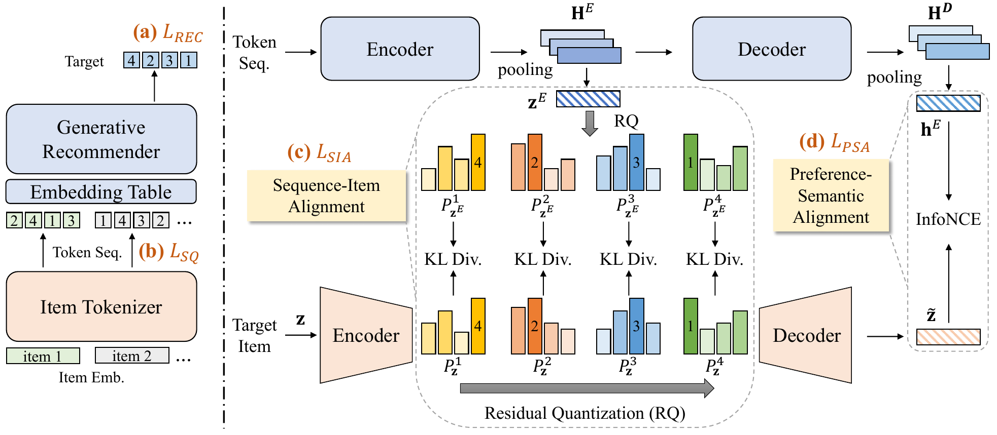
Figure 1 (Liu et al., 2024): The overall ETEGRec framework. The item tokenizer (bottom) performs residual quantization on item embeddings. The generative recommender (top) is a T5 encoder-decoder that processes the token sequence. SIA (left dashed box, panel c) aligns the encoder’s mean-pooled output \(\mathbf{z}^E\) with the target item’s codebook distributions via KL divergence at each quantization level. PSA (right dashed box, panel d) aligns the decoder’s first hidden state \(\mathbf{h}^D_0\) with the reconstructed item embedding \(\tilde{\mathbf{z}}\) via InfoNCE.
3. Recommendation-Oriented Alignment 🔑
The two alignment objectives are the core contribution. They differ in which representations they align and what signal they use.
3.1 Sequence-Item Alignment (SIA)
Motivation. The encoder’s hidden states \(\mathbf{H}^E\) summarize the user’s interaction history. If the encoder is well-trained, its mean-pooled output should represent “what kind of item the user wants next” — and this representation should produce similar codebook token distributions as the target item’s own embedding.
Construction. Apply mean pooling and an MLP to the encoder output:
\[\mathbf{z}^E = \text{MLP}(\text{MeanPool}(\mathbf{H}^E)) \in \mathbb{R}^{d_c}\]
Run \(\mathbf{z}^E\) through the same RQ-VAE residual quantization process to obtain predicted codebook distributions \(P^l_{\mathbf{z}^E}\) at each level \(l\). The target item’s embedding \(\mathbf{z}\) produces distributions \(P^l_{\mathbf{z}}\) via the same process.
Loss (symmetric KL divergence over all codebook levels):
\[\mathcal{L}_{\text{SIA}} = -\sum_{l=1}^L \left[D_{\text{KL}}\!\left(P^l_{\mathbf{z}} \,\|\, P^l_{\mathbf{z}^E}\right) + D_{\text{KL}}\!\left(P^l_{\mathbf{z}^E} \,\|\, P^l_{\mathbf{z}}\right)\right]\]
The symmetric KL (Jensen–Shannon-like) is used rather than one-directional KL to avoid the degenerate mode-seeking/mean-seeking failure modes of asymmetric divergences.
What SIA teaches the tokenizer. The gradient of \(\mathcal{L}_{\text{SIA}}\) with respect to codebook entries \(\mathbf{e}_k^l\) penalizes the tokenizer for assigning different code distributions to the target item and to the encoder’s prediction of “what the user wants.” Over many training steps, the codebook is pushed toward partitions where items that users actually transition to share similar codes — not just items that are similar in embedding space.
This question establishes what SIA’s gradient signal does to the codebook geometry.
Consider a simplified two-level RQ-VAE with codebook size \(K = 2\) and a single training example where the target item has \(P^1_\mathbf{z} = (0.9, 0.1)\) (strongly assigned to code 0) but the encoder predicts \(P^1_{\mathbf{z}^E} = (0.4, 0.6)\) (weakly preferring code 1). Compute the symmetric KL divergence for this level and state which component (\(\mathbf{z}\), \(\mathbf{z}^E\), or the codebook entries \(\mathbf{e}_k^1\)) receives the largest gradient magnitude. What does this imply about how SIA modifies the tokenizer vs. the recommender?
Key insight: \(D_{\text{KL}}((0.9,0.1) \| (0.4,0.6)) = 0.9 \ln(0.9/0.4) + 0.1 \ln(0.1/0.6) \approx 0.9(0.811) + 0.1(-1.792) \approx 0.551\). Symmetric KL \(\approx 0.551 + D_{\text{KL}}((0.4,0.6)\|(0.9,0.1)) \approx 0.551 + 0.4\ln(0.4/0.9) + 0.6\ln(0.6/0.1) \approx 0.551 + 0.4(-0.811) + 0.6(1.792) \approx 0.551 + 0.751 = 1.302\).
Sketch: The gradient flows into both the tokenizer (through \(P^l_\mathbf{z}\), which depends on the codebook entries \(\mathbf{e}_k^l\)) and the recommender encoder (through \(P^l_{\mathbf{z}^E}\), which depends on \(\mathbf{z}^E = \text{MLP}(\text{MeanPool}(\mathbf{H}^E))\)). However, during the tokenizer update phase (see §4), only the tokenizer parameters are unfrozen, so only the codebook receives gradient. SIA effectively tells the codebook: “when a user’s history predicts they want something like code 1, but the target item is code 0, that’s a penalty — try to assign the target item to a code that the recommender can predict.” The codebook thus reorganizes its clusters around behavioral similarity, not just embedding-space proximity.
3.2 Preference-Semantic Alignment (PSA)
Motivation. The decoder’s first hidden state \(\mathbf{h}^D_0 \in \mathbb{R}^d\) represents the model’s prediction of user preference before generating any output token. The reconstructed item embedding \(\tilde{\mathbf{z}} \in \mathbb{R}^{d_s}\) is the RQ-VAE’s best approximation of the target item. PSA aligns these two representations via contrastive learning.
Loss (InfoNCE with in-batch negatives):
\[\mathcal{L}_{\text{PSA}} = -\left[\log \frac{\exp(s(\tilde{\mathbf{z}}, \mathbf{h}^D_0) / \tau)}{\sum_{\hat{\mathbf{h}} \in \mathcal{B}} \exp(s(\tilde{\mathbf{z}}, \hat{\mathbf{h}}) / \tau)} + \log \frac{\exp(s(\mathbf{h}^D_0, \tilde{\mathbf{z}}) / \tau)}{\sum_{\hat{\mathbf{z}} \in \mathcal{B}} \exp(s(\mathbf{h}^D_0, \hat{\mathbf{z}}) / \tau)}\right]\]
where \(s(\cdot, \cdot)\) is cosine similarity, \(\tau\) is a temperature, and \(\mathcal{B}\) is the set of all in-batch items. The bidirectional form (two InfoNCE terms) mirrors CLIP’s symmetric contrastive objective.
SIA vs. PSA. The two objectives operate at different levels of the architecture:
| SIA | PSA | |
|---|---|---|
| Aligned representations | Encoder output ↔︎ item codebook distributions | Decoder first hidden state ↔︎ reconstructed item embedding |
| Signal type | Distributional (KL over token probabilities) | Geometric (cosine in embedding space) |
| Gradient target (tokenizer phase) | Codebook entries | RQ-VAE decoder (via \(\tilde{\mathbf{z}}\)) |
| Gradient target (recommender phase) | Encoder MLP | Decoder cross-attention |
PSA provides a coarser but more direct semantic alignment: the decoder’s user-preference vector should be geometrically close to the target item in reconstructed embedding space. SIA provides a finer distributional alignment between the encoder’s prediction and the item’s quantization structure.
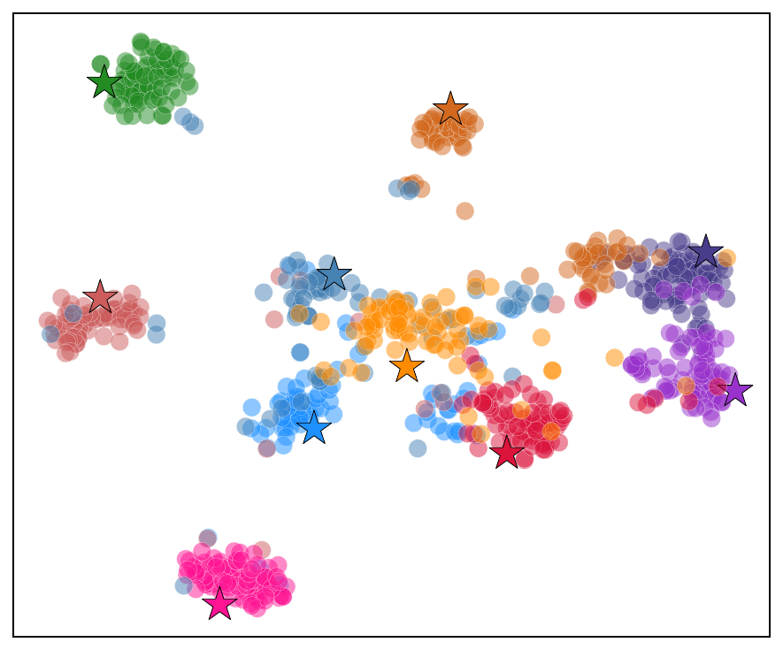
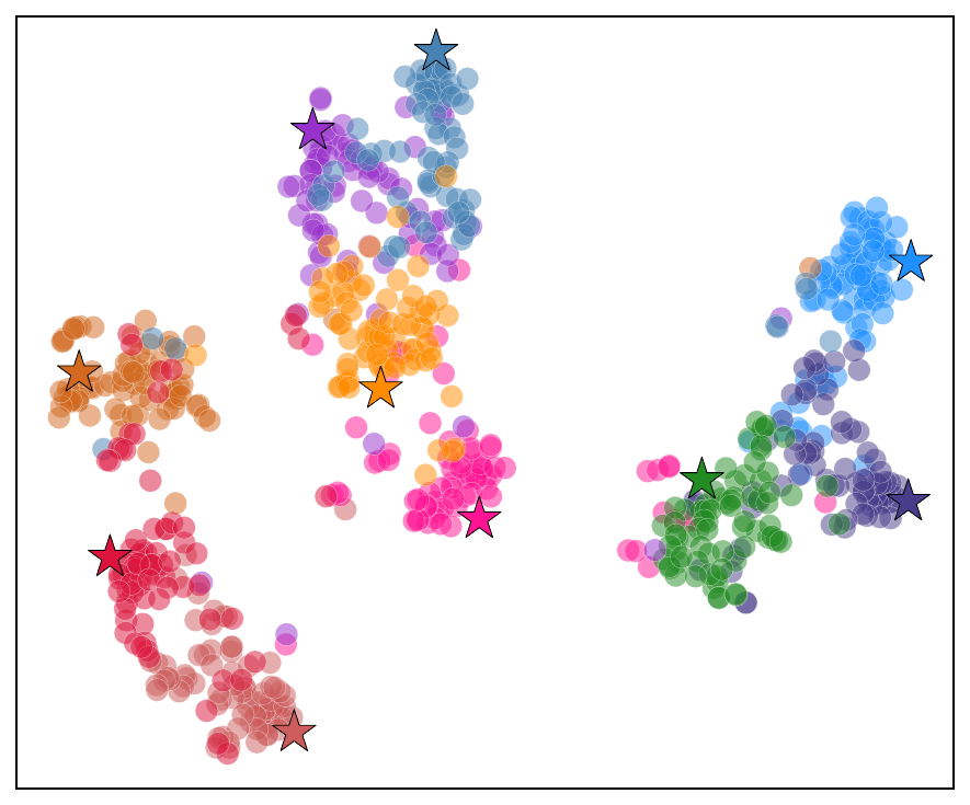
Figure 4 (Liu et al., 2024): t-SNE visualization of preference representations (\(\mathbf{h}^D_0\), circles) and semantic representations (\(\tilde{\mathbf{z}}\), stars) on Instruments (left) and Scientific (right). Each color denotes a distinct item group. After PSA training, preference points cluster near their corresponding semantic star, confirming that the decoder’s user-preference vector is geometrically aligned with the reconstructed target-item embedding.
4. Alternating Optimization ⚠️
ETEGRec alternates between two training phases in a cycle of 4 epochs:
Phase 1 — Tokenizer update (1 epoch, recommender frozen):
\[\mathcal{L}_{\text{IT}} = \mathcal{L}_{\text{SQ}} + \mu\, \mathcal{L}_{\text{SIA}} + \lambda\, \mathcal{L}_{\text{PSA}}\]
The RQ-VAE encoder, codebook entries, and decoder are updated. The recommender’s encoder-decoder weights are frozen. Gradients from \(\mathcal{L}_{\text{SIA}}\) reach the codebook via the tokenizer’s residual quantization; gradients from \(\mathcal{L}_{\text{PSA}}\) reach the RQ-VAE decoder via \(\tilde{\mathbf{z}}\).
Phase 2 — Recommender update (3 epochs, tokenizer frozen):
\[\mathcal{L}_{\text{GR}} = \mathcal{L}_{\text{REC}} + \mu\, \mathcal{L}_{\text{SIA}} + \lambda\, \mathcal{L}_{\text{PSA}}\]
The T5 encoder-decoder weights are updated. The RQ-VAE is frozen — semantic IDs are recomputed from the current tokenizer before each recommender epoch. Gradients from \(\mathcal{L}_{\text{SIA}}\) reach the encoder MLP; gradients from \(\mathcal{L}_{\text{PSA}}\) reach the decoder’s cross-attention and output layers.
The 1:3 ratio (one tokenizer epoch per three recommender epochs) reflects the different convergence rates: the tokenizer’s codebook is a discrete structure that converges quickly once the recommender provides a stable target; the recommender benefits from more gradient steps per tokenizer update.
Ablation on alternating training. Removing the alternating scheme (replacing it with simultaneous joint optimization) causes a −17.6% drop in Recall@5 on Instruments. This confirms that the sequential freeze-and-update discipline is necessary — not just a training heuristic — to prevent codebook destabilization.
This question examines the convergence properties of the alternating scheme.
Consider the alternating optimization as a two-block coordinate descent problem over parameters \((\theta_T, \theta_R)\) — tokenizer and recommender. The joint objective is \(\mathcal{L}(\theta_T, \theta_R) = \mathcal{L}_{\text{SQ}}(\theta_T) + \mathcal{L}_{\text{REC}}(\theta_R) + \mu\,\mathcal{L}_{\text{SIA}}(\theta_T, \theta_R) + \lambda\,\mathcal{L}_{\text{PSA}}(\theta_T, \theta_R)\). Under what conditions does alternating coordinate descent converge to a stationary point of \(\mathcal{L}\), and which of those conditions is most likely violated in practice?
Key insight: Block coordinate descent converges to a stationary point when (1) each block update finds a global minimum of \(\mathcal{L}\) over that block holding the other fixed, and (2) the joint objective is continuous and has bounded sublevel sets. In practice, neither holds: each phase uses SGD (not exact minimization), and \(\mathcal{L}_{\text{REC}}\) is non-convex. The most practically dangerous violation is condition (1): after each tokenizer update, the semantic IDs change, and the recommender’s next epoch must adapt to a shifted input distribution. If the tokenizer changes too fast relative to the recommender’s convergence speed, the recommender chases a moving target.
Sketch: The 1:3 epoch ratio is a practical heuristic to slow the tokenizer’s effective update rate. A more principled approach would be proximal updates (penalizing large changes to the tokenizer in each cycle) or setting a small learning rate for the tokenizer phase. Empirically, the paper validates the 1:3 ratio outperforms 1:1 and 1:5 ratios, suggesting the current schedule is near-optimal for the given architecture scale.
5. Experiments 📊
5.1 Overall Performance
Evaluation on three Amazon product review datasets:
| Dataset | Metric | SASRec | BERT4Rec | TIGER-SAS | ETEGRec |
|---|---|---|---|---|---|
| Baby | Recall@5 | 0.0209 | 0.0204 | 0.0233 | 0.0244 |
| Baby | NDCG@5 | 0.0136 | 0.0133 | 0.0151 | 0.0157 |
| Video Games | Recall@5 | 0.0485 | 0.0477 | 0.0558 | 0.0561 |
| Video Games | NDCG@5 | 0.0313 | 0.0305 | 0.0363 | 0.0365 |
| Instruments | Recall@5 | 0.0313 | 0.0308 | 0.0372 | 0.0385 |
| Instruments | NDCG@5 | 0.0197 | 0.0199 | 0.0240 | 0.0249 |
ETEGRec consistently leads, though margins over TIGER-SAS are modest (3–5% on most metrics). The largest gains appear on Instruments, the smallest on Video Games.
5.2 Ablation
| Variant | Instruments Recall@5 | Instruments NDCG@5 |
|---|---|---|
| ETEGRec (full) | 0.0385 | 0.0249 |
| w/o \(\mathcal{L}_{\text{SIA}}\) | 0.0383 | 0.0247 |
| w/o \(\mathcal{L}_{\text{PSA}}\) | 0.0377 | 0.0244 |
| w/o both alignment losses | 0.0370 | 0.0240 |
| w/o alternating training | 0.0317 | 0.0205 |
| w/o end-to-end (fixed tokenizer) | 0.0372 | 0.0238 |
Key observations: - Alternating training is by far the most important component. Removing it costs −17.6% Recall@5. This validates the core claim: end-to-end training requires the alternating discipline. - PSA contributes more than SIA (−2.1% vs. −0.5% on Recall@5). The geometric contrastive alignment provides a stronger gradient signal than the distributional KL. - Removing both alignment losses but keeping alternating training still underperforms the full model by −3.9% — confirming that the alignment objectives add value beyond simply enabling stable alternating updates.
5.3 Generalization to Cold-Start Users
On the 5% of users with the fewest historical interactions (coldest users), ETEGRec maintains its advantage over TIGER-SAS. The improvement is attributed to the decoder’s preference vector \(\mathbf{h}^D_0\) being aligned to item semantics via PSA, which provides a signal even when interaction history is sparse. A user with only 2–3 interactions has a noisy encoder output, but PSA ensures the decoder’s preference representation stays geometrically close to the relevant part of item space.
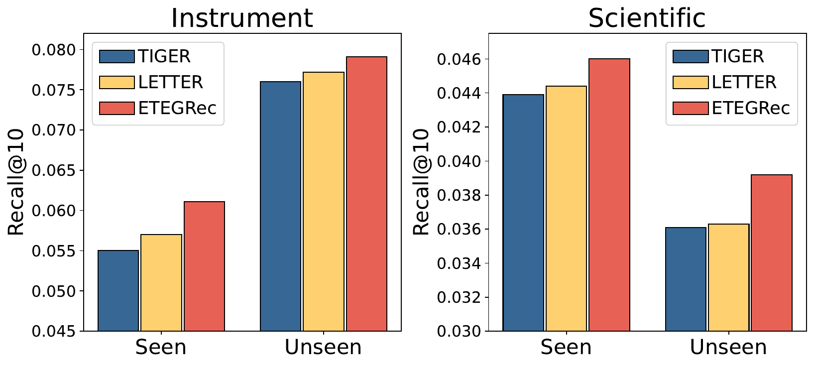
Figure 3 (Liu et al., 2024): Recall@10 for seen (training-set) and unseen (cold-start) users on Instruments (left) and Scientific (right). ETEGRec (red bars) leads on both seen and unseen splits. The gain on unseen users is larger in absolute terms on Scientific, consistent with the claim that PSA alignment provides a robust preference signal even for sparse interaction histories.
6. References
| Reference Name | Brief Summary | Link |
|---|---|---|
| ETEGRec: End-to-End Learnable Item Tokenization (Liu et al., 2024) | This paper | https://arxiv.org/abs/2409.05546 |
| TIGER: Recommender Systems with Generative Retrieval (Rajput et al., NeurIPS 2023) | Primary baseline; establishes the decoupled tokenization paradigm ETEGRec improves on | https://arxiv.org/abs/2305.05065 |
| VQ-VAE-2 (Razavi et al., 2019) | Hierarchical RQ-VAE construction underlying the item tokenizer | https://arxiv.org/abs/1906.00446 |
| Exploring the Limits of Transfer Learning with T5 (Raffel et al., 2020) | T5 encoder-decoder architecture used as the generative recommender backbone | https://arxiv.org/abs/1910.10683 |
| A Simple Framework for Contrastive Learning — SimCLR (Chen et al., 2020) | Contrastive InfoNCE objective used in PSA | https://arxiv.org/abs/2002.05709 |
| Self-Attentive Sequential Recommendation — SASRec (Kang & McAuley, 2018) | Sequential baseline; TIGER-SAS uses SASRec architecture with semantic IDs | https://arxiv.org/abs/1808.09781 |