Generative Reasoning Re-ranker (GR2)
Liang et al., Meta AI, 2026 · arXiv:2602.07774
| Dimension | Prior State | This Paper | Key Result |
|---|---|---|---|
| Reranking stage | Largely ignored in LLM-based recsys; focus on retrieval and ranking | Dedicated GR2 framework: LLM reasons over top-\(K\) candidates | +2.4% Recall@5, +1.3% NDCG@5 vs OneRec-Think |
| Item representation | Non-semantic IDs → vocabulary explosion for LLMs | RQ-VAE semantic IDs with ≥99% uniqueness via EMA + Random Last Level | EMA is the critical technique; alone lifts uniqueness from 31% → 97.5% |
| Reasoning training | SFT-only or zero-shot; reasoning potential untapped | Rejection-sampling SFT → DAPO RL with rank-promotion reward | RL is necessary; SFT alone often degrades R@1 |
| Reward hacking | Format rewards trivially exploited by copying pre-ranked order | Conditional format reward applied only when ranking actually improves | Closes the order-copying exploit |
Relations
Builds on: HSTU (Zhai et al., 2024), Wukong (Zhang et al., 2024) Concepts used: Generative Recommender Systems (§4.1 for semantic IDs, §5.3 for GR2 algorithm summary)
Table of Contents
- 1. What Problem Does GR2 Solve?
- 2. Stage 1 — Tokenized Mid-Training
- 3. Stage 2 — Reasoning Data Generation and SFT
- 4. Stage 3 — Reinforcement Learning with DAPO
- 5. Results
- 6. References
1. What Problem Does GR2 Solve? 🎯
Modern recommendation systems operate as a multi-stage funnel: from billions of items, a retriever narrows to thousands; a ranker further reduces to tens; and finally a reranker inspects the top few to decide the final order presented to the user. The reranker is the last quality gate — it sees the fewest candidates but has the highest impact on what the user actually experiences.
Prior LLM-based recommendation research focused almost entirely on retrieval and ranking, leaving reranking under-explored. What makes reranking special?
- Small candidate set. The reranker sees only \(K = 10\) pre-ranked candidates. This is small enough that an LLM can attend to all of them at once and reason about their relative ordering, rather than scoring each independently.
- Cross-candidate reasoning. A ranker predicts \(p(\text{action} \mid \text{user}, \text{item})\) for each candidate independently. A reranker can compare candidates against each other: “the user bought conditioner last week, so among these \(K\) candidates, the complementary item is X rather than Y.” This comparative signal is invisible to a scorer that sees one candidate at a time.
- Reasoning is uniquely valuable here. The small candidate set makes chain-of-thought reasoning tractable — the LLM can explicitly articulate why it promotes one candidate over another.
GR2 introduces a three-stage training pipeline to build a reasoning-capable reranker on top of a pretrained LLM (Qwen3-8B).
GR2 encodes items not as natural-language text descriptions but as semantic IDs — compact tuples of discrete codewords. This solves the scalability problem: an industrial item catalog has \(10^9\) items, and adding each as a natural-language string to the LLM’s context would be infeasible. Semantic IDs are short (4 tokens per item), learnable, and capture item semantics via the RQ-VAE training objective.
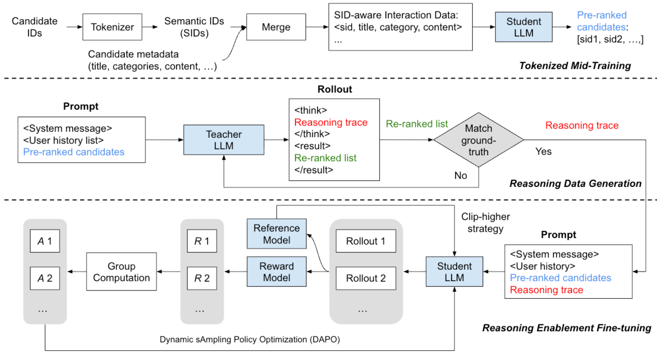
Figure 1 (Liang et al., 2026): Overview of the 3-stage training pipeline. Top: student LLM mid-training on tokenized semantic IDs (Tokenized Mid-Training). Middle: reasoning data generation with a teacher LLM and rejection sampling — rollouts are kept only when they match the ground-truth (Reasoning Data Generation). Bottom: student LLM reasoning enablement via SFT and DAPO RL, with group computation, reward model, and clip-higher strategy (Reasoning Enablement Fine-tuning).
2. Stage 1 — Tokenized Mid-Training 🏗️
Before the LLM can reason about items, it must understand items. A pretrained LLM knows language; it has never seen the notation <s_a_57><s_b_7><s_c_23><s_d_4> and has no idea that this represents a specific product in a catalog. Stage 1 solves this alignment problem.
2.1 Semantic IDs via RQ-VAE
Definition (Semantic ID). Given an item with textual features \(x\) (title, description, category), a Residual Quantized VAE (RQ-VAE) maps it to a tuple of discrete codeword indices:
\[\text{SID}(x) = (z_1, z_2, \ldots, z_K), \qquad z_k \in \{1, \ldots, C_k\}\]
where \(K\) is the number of quantization levels (GR2 uses \(K = 4\)) and \(C_k\) is the number of codewords in the \(k\)-th codebook. The construction proceeds residually: encode the item into a dense embedding \(\mathbf{h} = f_{\text{enc}}(x)\), then iteratively find the nearest codeword and subtract it:
\[z_k = \arg\min_{j} \|\mathbf{r}_k - \mathbf{e}_j^{(k)}\|_2, \quad \mathbf{q}_k = \mathbf{e}_{z_k}^{(k)}, \quad \mathbf{r}_{k+1} = \mathbf{r}_k - \mathbf{q}_k\]
where \(\mathbf{r}_1 = \mathbf{h}\). Each level refines the previous: level 1 captures the coarsest category (broad product type), level 4 captures fine-grained details. The reconstruction is \(\hat{\mathbf{h}} = \sum_k \mathbf{q}_k\).
The encoder and codebooks are trained jointly to minimize:
\[\mathcal{L} = \underbrace{\|\mathbf{h} - \hat{\mathbf{h}}\|_2^2}_{\text{reconstruction}} + \beta \sum_k \underbrace{\|\text{sg}[\mathbf{r}_k] - \mathbf{q}_k\|_2^2}_{\text{codebook loss}} + \gamma \sum_k \underbrace{\|\mathbf{r}_k - \text{sg}[\mathbf{q}_k]\|_2^2}_{\text{commitment loss}}\]
The sg[·] notation means stop-gradient: don’t backpropagate through this term. The codebook loss moves codebook entries toward inputs; the commitment loss moves encoder outputs toward codebook entries. The argmin in the forward pass is not differentiable, so gradients pass straight through it (the straight-through estimator).
Why this structure is useful for an LLM. Items with similar embeddings \(\mathbf{h}\) get similar semantic IDs — specifically, they share common prefix codes \((z_1, z_2, \ldots)\). Two conditioners are likely to share \((z_1, z_2)\) and differ only in \(z_3, z_4\). This hierarchy lets the LLM reason about item categories (shared prefixes) and individual items (full 4-tuples), the same way humans reason (“it’s a conditioner — specifically an Herbal Essences conditioner”).
2.2 Five Techniques for Codebook Quality
The fundamental pathology in RQ-VAE training is codebook collapse: codebook entries that are rarely selected receive no gradient signal, drift irrelevant, and eventually all inputs pile into the same few active entries. Collapsed codebooks cause SID collisions — two distinct items receiving the same 4-tuple — which makes the model unable to distinguish them.
GR2 tests five mitigation techniques in an ablation study. The results are stark:
Essential techniques (each contributes substantially):
🔑 EMA Codebook Updates. Instead of updating codebook entries via backpropagation, update them with an exponential moving average of the inputs assigned to each entry: \[\mathbf{e}_j^{(k)} \leftarrow \gamma\, \mathbf{e}_j^{(k)} + (1 - \gamma)\, \bar{\mathbf{r}}_j^{(k)}, \qquad \gamma \in [0.95, 0.99]\] where \(\bar{\mathbf{r}}_j^{(k)}\) is the mean of all level-\(k\) residuals assigned to entry \(j\) in the current batch. This bypasses the straight-through estimator entirely and gives codebook entries a direct, stable gradient signal. Ablation result: EMA alone lifts average uniqueness from 31.3% → 97.5% (+66.2%). This is the single most important technique.
🔑 Random Last Level. At inference time, assign the final quantization level \(z_K\) uniformly at random from unused codewords, rather than by nearest-neighbor. This sacrifices a small amount of reconstruction fidelity at the finest level in exchange for guaranteed distinctiveness. Ablation result: +28.7% uniqueness. All configurations achieving ≥99% uniqueness use this technique.
Optional techniques (marginal or negative):
Diversity Loss. Regularize codebook usage toward uniform distribution across entries. Adds +0.6% uniqueness — marginal, suggesting EMA already achieves sufficient coverage.
Dead Code Reset. Reinitialize unused codebook entries to items with the highest reconstruction error. Shows a slight negative effect (−4.0%), likely because resetting disrupts already-converged representations.
Contrastive Loss. Encourage co-interacted items to have similar embeddings. Counterintuitively hurts uniqueness (−13.2%) because items that are similar in user behavior intentionally share codes — increasing collision rate. However, it consistently improves downstream recommendation quality by encoding collaborative signal into the code structure.
Contrastive loss makes the model better at recommending but worse at distinguishing items (more collisions). This is not a contradiction: similar items sharing codes means beam search will find semantically related items more easily. The tradeoff is empirical — GR2’s best configuration enables contrastive loss (improves recommendation quality) while relying on EMA + Random Last Level for uniqueness.
| Technique | Uniqueness impact | Downstream rec. quality |
|---|---|---|
| EMA Updates | +66.2% (essential) | Neutral (infrastructure) |
| Random Last Level | +28.7% (essential) | Neutral |
| Contrastive Loss | −13.2% | Strong positive |
| Diversity Loss | +0.6% | Neutral |
| Dead Code Reset | −4.0% | Slightly negative |
2.3 Mid-Training: Bridging Item Tokens and Language
Once items have semantic IDs, GR2 adds new tokens <s_a_0> through <s_a_{C-1}>, etc. to the LLM’s vocabulary (one per codeword per codebook level), initializes their embeddings randomly, and mid-trains the LLM to understand them.
Training an LLM involves three distinct phases: - Pretraining: train from scratch on billions of tokens of internet text to learn general language, reasoning, and world knowledge. Enormously expensive ($10M+). The resulting model (e.g. Qwen3-8B) can answer general questions, write code, and reason about text. - Mid-training (also called continued pretraining or domain-adaptive pretraining): continue training the pretrained model on a new domain’s data — here, the “language” of item IDs interleaved with natural language. This is cheaper than pretraining but more expensive than fine-tuning. The goal is to teach the model a new vocabulary and its semantic structure without forgetting its original language abilities. - Fine-tuning / Post-training: train on specific tasks (Stage 2 and 3 below) with smaller learning rates and datasets.
GR2 follows the item alignment framework from OneRec-Think (Liu et al., 2025), training on four task types simultaneously:
| Task | What the model learns |
|---|---|
| Sequential Preference Modeling | Given a history of SIDs, predict the next SID |
| Itemic Dense Captioning | Given a SID, generate its natural-language description (title, categories) |
| Interleaved User Persona Grounding | Given a user’s SIDs and their reviews, model the user’s preferences |
| General Language Modeling | Standard next-token prediction on text — preserves existing language abilities |
The SID embedding table is optimized jointly with the rest of the model via the next-token prediction objective. By training on tasks that require the model to connect SIDs to natural language (Dense Captioning: <s_a_57>...<s_d_4> → “Stella McCartney Stella 1.7oz EDP Spray”), the model learns that SIDs are not arbitrary tokens but refer to real-world items.
Prompt: “Given an itemic token, generate a concise and accurate textual description. Token: <|sid_begin|><s_a_97><s_b_168><s_c_137><s_d_135><|sid_end|>”
Target output: “Title: Stella McCartney Stella. Description: STELLA For Women By STELLA MCCARTNEY 1.7 oz EDP Spray. Categories: Beauty > Fragrance > Women’s > Eau de Parfum”
After training on many such examples, the model learns that SIDs encode product semantics — their prefixes correspond to category clusters.
3. Stage 2 — Reasoning Data Generation and SFT 📚
3.1 What is Supervised Fine-Tuning?
Supervised Fine-Tuning (SFT) is the most straightforward way to teach a pretrained LLM to behave in a specific way. The idea:
- Collect a dataset of (input, desired output) pairs. The “desired output” is the exact text you want the model to produce for a given input.
- Train the model with standard cross-entropy loss: for each token in the desired output, minimize \(-\log P(\text{token} \mid \text{prior context})\).
- The model learns to produce outputs that look like the demonstrations.
The key limitation. SFT only teaches the model to imitate the demonstration outputs. If the demonstrations contain a step-by-step reasoning trace that correctly identifies the next purchase, the model learns to generate reasoning traces that look like those — but it doesn’t necessarily learn that the goal is to actually rank the correct item highest. SFT optimizes format and fluency; it does not directly optimize ranking accuracy. This is why GR2 needs RL in Stage 3.
In recommendation: an SFT-trained model might produce a beautiful, coherent reasoning trace that nonetheless ranks the wrong item first.
3.2 Generating the Training Data: Rejection Sampling
The central challenge for SFT is: where do the (input, desired output) pairs come from? Human annotation of reasoning traces for millions of recommendations would be infeasible. GR2 uses a teacher LLM (Qwen3-32B, a larger, more capable model) to generate the training data automatically.
Two strategies are compared:
Targeted sampling. Provide the teacher LLM with the user’s history, the candidate list, and the ground-truth next item, and ask it to generate a reasoning trace explaining why that item is the right choice:
\[\tau \sim P_\theta\!\left(\cdot \mid P_{\text{targeted}}(\text{history},\, \text{candidates},\, \text{ground truth item})\right)\]
Since the answer is given, the teacher always produces a trace — but it may produce post-hoc rationalization without genuine reasoning.
Rejection sampling. Do not reveal the ground truth. Ask the teacher to predict which candidate the user will choose. Keep sampling until the teacher’s prediction matches the ground truth:
\[(\tau, \hat{y}) \sim P_\theta\!\left(\cdot \mid P_{\text{rejection}}(\text{history},\, \text{candidates})\right) \quad \text{subject to } \hat{y} = y^*\]
The constraint “keep only traces where the model predicted correctly” acts as a filter. Only traces where the reasoning actually led to the right answer are kept. This means the SFT data contains chains of thought that the teacher genuinely believed, not just plausible-sounding confabulations. The training signal is cleaner: the model learns that good reasoning correlates with correct predictions.
The tradeoff: rejection sampling is slower (may require many samples to find a correct prediction) and may be biased toward “easy” examples where the teacher predicts correctly on the first try.
Prompt engineering principles. Five principles shape the prompts sent to the teacher LLM:
- Domain knowledge priming: explicitly inject e-commerce heuristics (“consider sequential purchase patterns like shampoo → conditioner → styling products”) to guide the reasoning structure
- SID citation requirement: force the model to cite items by their SID tokens — this prevents vague references and makes traces verifiable
- Collaborative context: present the full history and all candidates simultaneously, enabling holistic comparison
- Structured step format: require a hierarchical structure — (1) broad pattern recognition, (2) complementary product identification, (3) final candidate selection
- Structured JSON output: require both the reasoning trace and the ranked list in a parseable format
3.3 The SFT Loss
Each training example is a three-part chat message (system prompt + user message + assistant message). The model is trained to generate the assistant message — which contains both the reasoning trace \(\tau = [r_1, \ldots, r_M]\) and the ranked output \(o = [o_1, \ldots, o_T]\).
Two separate loss weights are applied:
\[\mathcal{L}_{\text{SFT}} = -\lambda_r \sum_{i=1}^M \log P(r_i \mid \mathcal{P}, r_{<i}) - \lambda_o \sum_{j=1}^T \log P(o_j \mid \mathcal{P}, \tau, o_{<j})\]
with \(\lambda_r < \lambda_o\). The ranking output tokens are weighted more heavily than the reasoning tokens. This decoupling prevents a failure mode where the model learns to generate fluent reasoning at the expense of ranking accuracy — the reasoning tokens see lower gradient weight, so they serve as a scaffold rather than the primary learning target.
Empirical results in Table 5 show that SFT-targeted models (with domain knowledge priming, “KP”) actually decrease recall@1 vs the pre-ranked baseline (0.2006 vs 0.2892). The SFT model produces coherent-looking reasoning but does not consistently promote the right item. The mismatch between “good-looking reasoning trace” and “high ranking accuracy” is real and quantitatively significant. RL is needed to directly optimize what actually matters.
4. Stage 3 — Reinforcement Learning with DAPO 🤖
4.1 Why SFT Alone Is Not Enough
SFT trains the model by minimizing the cross-entropy loss against fixed demonstration outputs. This has two structural problems for reranking:
Imitation ≠ optimization. SFT teaches the model to produce outputs that look like the demonstrations. But a reasoning trace that leads to a slightly wrong ranking is penalized identically to one that is completely wrong. The loss function has no notion of “how much better” one ranking is over another.
Distribution shift. During SFT, the model sees the teacher’s demonstrations. During inference, it generates its own outputs. Errors compound: a token generated slightly differently from the demonstration puts the model into a context it was never trained on.
RL directly addresses both: it evaluates the model’s own outputs against a reward signal, with no reference to demonstrations.
4.2 Reinforcement Learning for LLMs: The Core Idea
In reinforcement learning, an agent takes actions in an environment and receives rewards. The goal is to learn a policy — a mapping from situations to actions — that maximizes expected cumulative reward.
For LLMs: - The policy \(\pi_\theta\) is the LLM parameterized by weights \(\theta\): given input text (a prompt), it produces output text (a response). - Each action is generating the next token. - The environment is the task: given a user history and candidate list, re-rank the candidates. - The reward is a scalar evaluating the full generated output: did the model promote the right item? Is the output parseable JSON?
The fundamental challenge: unlike supervised learning, the reward is only observed after the full sequence is generated. There is no per-token label — the entire sequence either succeeds or fails. This is the credit assignment problem: which tokens caused the good/bad outcome?
Policy gradient methods solve this by estimating the expected gradient of the reward with respect to the policy: \[\nabla_\theta J(\theta) = \mathbb{E}_{\tau \sim \pi_\theta}\!\left[\sum_t \nabla_\theta \log \pi_\theta(a_t \mid s_t) \cdot R(\tau)\right]\] where \(R(\tau)\) is the total reward for sequence \(\tau\). Intuitively: if a sequence gets a high reward, increase the probability of every action in that sequence; if it gets a low reward, decrease them. This is the REINFORCE algorithm (Williams, 1992).
Why we can’t use plain REINFORCE. The gradient estimator has high variance (lucky sequences get rewarded even if most of their tokens were irrelevant) and can lead to large, destabilizing updates. Modern LLM RL algorithms add three key ingredients: (1) a baseline to reduce variance, (2) a clipping mechanism to prevent large updates, and (3) a KL penalty to prevent the model from drifting too far from its starting point.
4.3 GRPO: Group Relative Policy Optimization
GRPO (Shao et al., 2024, from the DeepSeekMath paper) provides the algorithmic foundation for DAPO. The key idea is to replace the critic/value network used in PPO with a group baseline.
Setup. For each training prompt \(q\) (a user history + candidate list), sample a group of \(G\) output sequences \(\{o_i\}_{i=1}^G\) from the current policy \(\pi_{\theta_{\text{old}}}\). Evaluate each with the reward function: \(R_1, \ldots, R_G\).
Group-normalized advantage. The advantage of output \(i\) relative to the group is: \[\hat{A}_i = \frac{R_i - \text{mean}(\{R_j\}_{j=1}^G)}{\text{std}(\{R_j\}_{j=1}^G)}\]
This is the baseline: instead of estimating how good state \(s\) is via a learned value function (PPO), GRPO estimates it by comparing output \(i\) to the other \(G-1\) outputs sampled from the same prompt. If \(R_i\) is above the group average, \(\hat{A}_i > 0\) (this was a good output, increase its probability); if below, \(\hat{A}_i < 0\) (decrease its probability).
The high variance in policy gradient estimates comes from the fact that some prompts are inherently hard (low reward regardless of the output) and some are easy. A global baseline (average reward over the dataset) doesn’t account for this. By comparing within a group sampled from the same prompt, the advantage estimate captures “was this output better than average for this prompt?” — much lower variance than comparing against a global average.
The PPO-clip objective. To prevent large, destabilizing policy updates, GRPO uses PPO-style clipping. The importance ratio \(r_{i,t}(\theta) = \pi_\theta(o_{i,t} \mid q, o_{i,<t}) / \pi_{\theta_{\text{old}}}(o_{i,t} \mid q, o_{i,<t})\) measures how much the current policy differs from the old policy at token \(t\) of output \(i\). The clipped objective:
\[J_{\text{GRPO}}(\theta) = \mathbb{E}\!\left[\frac{1}{G} \sum_{i=1}^G \frac{1}{|o_i|} \sum_{t=1}^{|o_i|} \min\!\left(r_{i,t}(\theta)\hat{A}_{i,t},\, \text{clip}(r_{i,t}(\theta), 1-\varepsilon, 1+\varepsilon)\hat{A}_{i,t}\right)\right]\]
The clip prevents the importance ratio from exceeding \([1-\varepsilon, 1+\varepsilon]\), which bounds the size of any single gradient step. If the current policy wants to make a large update (ratio far from 1), the clipping cuts the gradient signal, preventing destabilization.
4.4 DAPO: Two Extensions to GRPO
DAPO (Decoupled Clip and Dynamic sAmpling Policy Optimization, Yu et al., 2025) extends GRPO with two modifications that address specific failure modes observed in practice.
Modification 1: Clip-Higher (decoupled clip thresholds). Standard GRPO uses the same \(\varepsilon\) for both positive and negative clipping. DAPO decouples them:
\[\text{clip}(r_{i,t}(\theta),\, 1 - \varepsilon_{\text{low}},\, 1 + \varepsilon_{\text{high}})\]
Typically \(\varepsilon_{\text{high}} > \varepsilon_{\text{low}}\), allowing larger increases in probability for good outputs than decreases for bad ones. The motivation: when the policy has found a good reasoning trace, it should be able to reinforce it strongly; overly tight upper clipping prevents useful positive updates.
Modification 2: Dynamic sampling (filtering degenerate prompts). A degenerate prompt is one where all \(G\) sampled outputs produce the same reward — either all correct (accuracy = 1) or all incorrect (accuracy = 0). In both cases, \(\hat{A}_i = 0\) for all \(i\) (all rewards are equal, so the advantage is zero after normalization). Zero advantage → zero gradient → no learning.
DAPO filters out these prompts:
\[\text{subject to } 0 < \left|\{o_i \mid \text{is\_correct}(o_i)\}\right| < G\]
Only prompts where some but not all outputs are correct contribute to training. These are the informative prompts: the model is at the learning frontier — sometimes getting it right, sometimes not — and the group advantage can distinguish good from bad outputs.
\[J_{\text{DAPO}}(\theta) = \mathbb{E}_{(q,D)\sim\mathcal{D},\, \{o_i\}_{i=1}^G \sim \pi_{\theta_{\text{old}}}}\!\left[\frac{1}{G} \sum_{i=1}^G \frac{1}{|o_i|} \sum_{t=1}^{|o_i|} \min\!\left(r_{i,t}(\theta)\hat{A}_{i,t},\; \text{clip}(r_{i,t}(\theta), 1{-}\varepsilon_{\text{low}}, 1{+}\varepsilon_{\text{high}})\hat{A}_{i,t}\right)\right]\] subject to \(0 < |\{o_i \mid \text{is\_equivalent}(\hat{y}, o_i)\}| < G\)
4.5 The Ranking Reward
The task is to re-rank a pre-ranked candidate list of \(|D|\) items so that the ground-truth next item \(x^*\) moves higher. The reward directly measures this:
\[R_{\text{rank}} = \frac{\text{rank}_{\text{pre}}(x^*) - \text{rank}_{\text{re}}(x^*)}{|D|}\]
where \(\text{rank}_{\text{pre}}\) is the item’s position in the pre-ranked list (from the retriever) and \(\text{rank}_{\text{re}}\) is its position in the re-ranked list (from the LLM). A positive reward means the target item was promoted; a negative reward means it was demoted. The normalization by \(|D|\) keeps rewards in \([-1, 1]\).
Suppose \(|D| = 10\). The retriever’s pre-ranked list has the ground-truth item at position 4. If GR2 re-ranks it to position 1: \(R_{\text{rank}} = (4 - 1)/10 = 0.3\). If GR2 demotes it to position 7: \(R_{\text{rank}} = (4 - 7)/10 = -0.3\).
4.6 Conditional Format Reward and Reward Hacking
GR2 also needs the model to produce parseable output — a valid JSON object with both a reasoning trace and a ranked list. A format reward \(R_{\text{fmt}} = \Omega(o)\) checks whether the output parses correctly.
The reward hacking problem. If both rewards are combined naively — \(R = R_{\text{rank}} + \alpha R_{\text{fmt}}\) — the model finds a degenerate strategy: copy the pre-ranked order unchanged. This guarantees: - \(R_{\text{rank}} = 0\) (no demotion, no promotion) - \(R_{\text{fmt}} > 0\) (the output is still a valid ranked list in JSON)
Net reward: \(0 + \alpha > 0\). The model has learned to do nothing and still collect positive reward. This is the classic reward hacking failure mode in RL: the model satisfies the reward function without achieving the intended objective.
The fix: conditional format reward.
\[R = \begin{cases} R_{\text{rank}} + \alpha R_{\text{fmt}} & \text{if } R_{\text{rank}} > 0 \text{ or } \text{rank}_{\text{pre}}(x^*) = 1 \\ R_{\text{rank}} & \text{otherwise} \end{cases}\]
The format reward is only added when the ranking actually improved (\(R_{\text{rank}} > 0\)), or when the item was already at rank 1 (the model can’t improve further, so format quality should still be rewarded). In all other cases — including the order-copying exploit — the model only receives the negative ranking reward. This closes the loophole.
The order-copying exploit is a specific instance of a general principle: whenever a reward function has multiple components, the model will find the lowest-effort path to positive total reward, which may involve doing nothing useful on the hardest component while maximizing the easiest. Conditional rewards (applying component \(B\) only when component \(A\) already succeeds) are a principled countermeasure. DeepSeek-R1, DAPO, and GR2 all use variants of this pattern.
5. Results 📊
On Amazon Beauty and Sports datasets (Table 5/6):
| Configuration | R@1 | R@5 | NDCG@5 |
|---|---|---|---|
| Pre-rank baseline (MTL) | 0.2892 | 0.7227 | 0.5101 |
| SFT-targeted-KP | 0.2006 | 0.7250 | 0.4759 |
| SFT-rejection-KP | 0.2784 | 0.7091 | 0.4970 |
| RL-targeted-KP | 0.2898 | 0.7221 | 0.5101 |
| RL-rejection-KP (best) | 0.2977 | 0.7460 | 0.5234 |
Key findings from ablations:
1. SFT alone often hurts R@1. SFT-targeted-KP drops R@1 from 0.2892 to 0.2006 — a regression from the pre-ranked baseline. The model learns to produce coherent reasoning but does not reliably promote the right item. This directly motivates Stage 3.
2. RL recovers and surpasses the baseline. RL-rejection-KP achieves R@1 = 0.2977 (+2.9% over baseline) and R@5 = 0.7460 (+3.2% over baseline). The ranking reward directly optimizes what matters.
3. Rejection sampling > targeted sampling. RL-rejection-KP outperforms RL-targeted-KP across all metrics. Rejection-sampled traces — where the teacher genuinely predicted the right answer without being told — provide cleaner supervision than post-hoc rationalization.
4. Domain knowledge priming matters. Comparing KP vs noKP variants under the same RL setting: RL-rejection-KP (0.5234 NDCG@5) vs RL-rejection-noKP (0.5172 NDCG@5). The sequential purchase heuristics (“shampoo → conditioner → styling”) injected into prompts encode domain knowledge that improves the reasoning quality even after RL fine-tuning.
Comparison with OneRec-Think (SOTA): GR2 surpasses OneRec-Think by +2.4% Recall@5 and +1.3% NDCG@5 on the Amazon datasets.
6. References
| Reference Name | Brief Summary | Link |
|---|---|---|
| GR2: Generative Reasoning Re-ranker (Liang et al., Meta 2026) | Three-stage LLM reranker: tokenized mid-training → rejection-sampling SFT → DAPO RL; conditional format reward prevents order-copying exploit | https://arxiv.org/abs/2602.07774 |
| DAPO: Decoupled Clip and Dynamic Sampling Policy Optimization (Yu et al., 2025) | Extends GRPO with Clip-Higher (separate ε_low, ε_high) and dynamic prompt filtering; resolves entropy collapse and zero-gradient degenerate cases | https://arxiv.org/abs/2503.14476 |
| DeepSeekMath / GRPO (Shao et al., 2024) | Introduces Group Relative Policy Optimization: group-normalized advantage replaces learned critic; enables scalable RL for LLMs without a separate value model | https://arxiv.org/abs/2402.03300 |
| OneRec-Think (Liu et al., 2025) | Introduces item alignment mid-training stage for generative LLM recommendation; four alignment tasks; GR2 inherits and improves on this design | https://arxiv.org/abs/2510.11639 |
| TIGER: Recommender Systems with Generative Retrieval (Rajput et al., NeurIPS 2023) | First semantic ID approach for generative recommendation via RQ-VAE | https://arxiv.org/abs/2305.05065 |
| Autoregressive Image Generation Using Residual Quantization / RQ-VAE (Lee et al., CVPR 2022) | Foundational RQ-VAE architecture underlying semantic ID construction in GR2 and TIGER | https://arxiv.org/abs/2203.01941 |
| Chain-of-Thought Prompting (Wei et al., NeurIPS 2022) | Establishes chain-of-thought as a general technique for eliciting multi-step reasoning from LLMs | https://arxiv.org/abs/2201.11903 |
| Qwen3 Technical Report (Qwen Team, 2025) | Base model (8B and 32B variants) used as student and teacher LLMs in GR2 | https://arxiv.org/abs/2505.09388 |