Actions Speak Louder than Words: Trillion-Parameter Sequential Transducers for Generative Recommendations
Jiaqi Zhai, Lucy Liao, Xing Liu, Yueming Wang, Rui Li, Xuan Cao, Leon Gao, Zhaojie Gong, Fangda Gu, Michael He, Yinghai Lu, Yu Shi. Meta Platforms, Inc. arXiv 2402.17152, February 2024.
| Dimension | Prior State | This Paper | Key Result |
|---|---|---|---|
| Recommendation paradigm | Impression-level DLRM: each (user, item) pair scored independently; heterogeneous feature engineering | Sequential transduction: user history as time series; single generative forward pass covers retrieval and ranking | +12.4% engagement (ranking), +6.2% retrieval HR@100 |
| Architecture | DLRMs with FM-like interactions over static features; Transformers unstable on industrial streaming data | HSTU: Transformer variant with pointwise attention (no softmax), temporal relative bias, and fused SiLU gating | Stable training at 1.5T params; NaN-free on industrial streaming data |
| Scale | DLRM plateau ~200B params; Transformer NaN loss on industrial data | 1.5 trillion parameters; stable training; scaling law across 3 orders of magnitude | Power-law scaling holds across 3 orders of magnitude in FLOPs |
| Inference cost | Linear in candidates; no amortization across candidates | M-FALCON: O(n²d) amortized across \(b_m\) candidates via modified attention masks | 285× model complexity at 1.5–2.5× throughput improvement |
| Training efficiency | Impression-level: O(N³d) complexity | Generative with stochastic length: O(N^α d), α ∈ (1,2]; 5.3–15.2× faster than FlashAttention2 | 5.3–15.2× faster than FlashAttention2 on 8192-length sequences |
| Online performance | Baselines | +12.4% engagement (ranking), +6.2% retrieval HR@100; deployed serving billions of users | Deployed to billions of users; largest reported rec-sys gains |
Relations
Builds on: DHEN Extended by: Wukong, SlimPer Concepts used: A/B Testing Foundations, Standard Attention
Table of Contents
- 1. Motivation and Background
- 2. Sequence Representation
- 3. HSTU Architecture
- 4. Computational Efficiency
- 5. Scaling Laws
- 6. Experiments
- 7. Relation to Wukong
- 8. References
1. Motivation and Background
1.1 Limitations of DLRM-Style Systems
Deep Learning Recommendation Models (DLRMs) process each (user, item) impression independently: given a user context \(u\) and candidate item \(x\), they output \(p(\text{click} \mid u, x)\). The pipeline requires:
- Extensive feature engineering: hand-crafted numerical features (recency, click-through rates, session counts) in addition to raw categorical IDs.
- Impression-level training: each example in the training batch is one (user, item, label) triple. For a user with \(n_i\) historical interactions, scoring all items requires \(n_i\) separate forward passes.
- Separate models for retrieval and ranking: different architectures, training pipelines, and feature sets.
These choices introduce fundamental scalability barriers: - Feature engineering is human-bottlenecked: numerical features capture only what engineers think to measure. - Impression-level training complexity scales as \(O(N^3 d)\) where \(N = \max_i n_i\) is the maximum sequence length (shown in Section 4.1). - Separate retrieval/ranking pipelines double infrastructure cost and prevent knowledge transfer between stages.
Why DLRMs fail to scale with compute (Zhao et al., 2023). The HSTU paper cites Zhao et al. (KDD 2023) as empirical grounding for the scaling failure. Their paper identifies a precise mechanism they term quality saturation: DLRM-style systems that represent items with per-ID embeddings (item-centric ranking, ICR) encounter a parameter explosion as the item inventory grows.
On creator-economy platforms (feeds, short video), the item inventory grows linearly over time: \(|\mathcal{I}| = O(t)\). Total parameter count therefore grows as:
\[\text{params}(t) = \text{const} + |\mathcal{I}(t)| \cdot d\]
Meanwhile, the total training data volume grows only as \(O(t)\) as well — so the training signal per parameter stays constant rather than improving. Zhao et al. show this leads to a hard asymptotic error floor:
\[\mathbb{E}\left[\|\hat{\theta}_t - \theta^*\|^2\right]_{\text{ICR}} = \Omega(1) \quad \text{as } t \to \infty\]
compared to \(O(1/t)\) for their proposed user-centric alternative. This is not a data problem — it holds even as training data grows without bound. The parameter count simply outruns the available training signal because item embeddings are ephemeral: items leave the inventory (videos deleted, ads expired), and their embeddings accumulate signal briefly before becoming irrelevant. The model cannot amortize compute over a stable vocabulary the way LLMs amortize over a fixed token set.
Concretely, at 60 days of training data, an ICR model is 21× larger in total parameters than a user-centric counterpart trained on identical data — yet achieves worse metric performance. Increasing embedding dimension (a direct proxy for model capacity and compute) causes ICR to degrade in production experiments (Table 4 of Zhao et al.), while the user-centric model continues to improve. Distribution drift compounds the problem: model quality degrades significantly within 24 hours of training cutoff on fast-moving item distributions, so additional compute invested in a larger ICR model depreciates rapidly.
HSTU’s response to this analysis is to abandon per-item embeddings as the primary modeling unit and instead treat recommendation as sequential transduction over a bounded, dense user action space — sidestepping the parameter explosion entirely.
1.2 Why Standard Transformers Fail on Recommendation Data
The natural candidate for replacing DLRMs is the Transformer, which already models sequential data via self-attention. However, naively applying Transformers to industrial recommendation data fails for three reasons:
Non-stationarity. User interests shift over time; the item vocabulary changes continuously (new items appear, old ones disappear). Standard Transformers assume a fixed vocabulary and stationary distribution. The non-stationary vocabulary makes softmax attention counterproductive (see Section 3.4).
High cardinality. Recommendation vocabularies contain billions of items. Unlike NLP (50K tokens), the embedding matrix alone can exceed terabytes.
Numerical instability. On industrial streaming data with variable sequence lengths and non-stationary distributions, Transformers produce NaN loss during training (Table 4 shows this empirically — Transformers fail outright on the industrial streaming task).
1.3 The Generative Recommender Paradigm
HSTU reformulates recommendation as sequential transduction: given the user’s history \(h = (x_0, x_1, \ldots, x_{n-1})\) as an ordered time series, predict the next item \(x_n\) (retrieval) or the action \(a_n\) the user will take on item \(x_n\) (ranking).
This shift has three consequences:
- Unified model: a single encoder handles both retrieval (next-item prediction) and ranking (next-action prediction) in the same forward pass.
- Training efficiency: a single sequence generates many training signals (one per history position), eliminating the need for impression-level batching.
- Feature simplification: raw categorical IDs in chronological order replace engineered numerical features.
2. Sequence Representation
2.1 Unified Time Series
All user interactions are merged into a single chronological time series. Each event is represented by its item embedding \(\mathbf{x}_t \in \mathbb{R}^d\) (from an item ID lookup). Numerical features such as click-through rates, session statistics, and dwell times are removed — the model is expected to infer these implicitly from the action sequence itself.
The sequence for user \(i\) is:
\[h_i = (x_0, x_1, \ldots, x_{n_i - 1}) \in \mathbb{R}^{n_i \times d}\]
Aside: what does “target-aware” mean? In recommendation, you’re always scoring a specific candidate item (the “target”) against a user’s history. A model is target-aware if the user representation it computes depends on which candidate is being scored. A context-free model sum-pools history into one fixed vector \(\mathbf{u}\) used identically for every candidate. A target-aware model recomputes \(\mathbf{v}_U(A)\) per candidate, upweighting history items semantically related to \(A\) and downweighting irrelevant ones — so the same user appears different when scoring a tennis racket vs. a laptop. This is strictly more expressive than any static numerical feature, which commits to a fixed aggregation at engineering time.
Why removing numerical features is justified: the DIN argument (Zhou et al., 2018). This design choice rests on an observation from the Deep Interest Network paper: the role that handcrafted numerical features play is to summarize the relevance of a user’s behavioral history to the candidate item being scored. Typical features include:
- Weighted/decayed counters: “number of clicks on sports items in the past 7 days” (approximates recent interest in a category)
- Engagement ratios: \(\text{CTR} = \frac{\text{clicks on category } c}{\text{impressions on category } c}\) (approximates preference intensity per category)
- Aggregated cross-product features: clicks broken down by (category, brand, price tier) to capture fine-grained preference slices
All of these are fixed, pre-computed aggregations over the raw history — they collapse the sequence into a scalar or small vector that human engineers believe is informative. The fundamental limitation is that they are context-free: a feature like “7-day sports CTR” is the same regardless of whether the current candidate is a tennis racket or running shoes.
DIN replaces static pooling with a local activation unit that produces a candidate-conditioned user representation:
\[\mathbf{v}_U(A) = \sum_{j=1}^{H} a(\mathbf{e}_j,\, \mathbf{v}_A)\cdot \mathbf{e}_j\]
where \(\mathbf{v}_A\) is the candidate item embedding, \(\{\mathbf{e}_j\}\) are history item embeddings, and the scalar weights \(a(\mathbf{e}_j, \mathbf{v}_A)\) are output by a small MLP applied to the concatenation \([\mathbf{e}_j,\ \mathbf{v}_A,\ \mathbf{e}_j \odot \mathbf{v}_A,\ \mathbf{e}_j \otimes \mathbf{v}_A]\). The outer product term \(\mathbf{e}_j \otimes \mathbf{v}_A\) gives the network explicit access to cross-item feature interactions. Crucially, the weights are not softmax-normalized — the magnitude of \(\mathbf{v}_U(A)\) encodes preference intensity, not just relative attention.
The consequence is that DIN subsumes numerical aggregates: the model can learn to selectively upweight the subset of history behaviors semantically related to the candidate, dynamically recomputing what a “sports CTR” counter would have captured but conditioned on the specific candidate at inference time. This is strictly more expressive — it adapts the aggregation to each candidate rather than committing to a single feature partition at feature engineering time.
HSTU extends this logic to its limit: given a sufficiently expressive sequential transducer (HSTU layers stacked to 1.5T parameters) operating over the full user history, the model can implicitly recompute arbitrary candidate-conditioned aggregations that any handcrafted numerical feature encodes — while also capturing higher-order temporal patterns no static feature could represent. At scale, the raw action sequence is informationally richer than any fixed derived feature set.
2.2 Retrieval vs. Ranking Formulation
Retrieval task. Given history \(h_i\) up to position \(t\), the model produces a hidden state \(u_t \in \mathbb{R}^d\) and scores all content items:
\[\text{retrieve: } \arg\max_{x \in \mathcal{X}_c} p(x \mid u_t)\]
where \(\mathcal{X}_c\) is the content item vocabulary. Training uses a masked language modeling objective: at each position \(t\), predict \(x_{t+1}\) from \(u_t\). A mask \(m_t = 0\) when the output is undefined (e.g., non-engagement actions like impressions without clicks).
Ranking task. Item events and action events are interleaved:
\[h_i^{\text{rank}} = (x_0, a_0, x_1, a_1, \ldots, x_{n-1}, a_{n-1})\]
where \(a_t \in \{0, 1\}\) (or a richer action space) is the user’s response to item \(x_t\). During ranking inference, the target item \(x_{\text{target}}\) is appended, and the model attends over the full history to predict \(a_{\text{target}}\). This target-aware cross-attention is handled in a single forward pass by including the target in the sequence with a special mask.
3. HSTU Architecture
The Hierarchical Sequential Transduction Unit (HSTU) is a single block that replaces the Transformer block. Each HSTU layer applies three sub-layers in sequence:
3.1 Sub-Layer 1: Pointwise Projection
\[U(X),\ V(X),\ Q(X),\ K(X) = \text{Split}\!\left(\varphi_1\!\left(f_1(X)\right)\right)\]
where: - \(f_1(X) = W_1 X + b_1\) is a single linear projection expanding the embedding dimension by 4×. - \(\varphi_1\) is the SiLU (Sigmoid Linear Unit) nonlinearity: \(\text{SiLU}(z) = z \cdot \sigma(z)\). - \(\text{Split}\) partitions the 4×-expanded projection into four equal parts: \(U, V, Q, K \in \mathbb{R}^{n \times d}\).
Motivation: The four-way split separates the representation into two roles: - \(Q, K\) are used for spatial aggregation (computing attention weights). - \(U\) is used for gating after aggregation. - \(V\) is used for value aggregation.
The SiLU nonlinearity (rather than ReLU) provides smooth gating behavior and was empirically found to stabilize training on non-stationary data.
3.2 Sub-Layer 2: Spatial Aggregation
\[A(X) V(X) = \varphi_2\!\left(Q(X) K(X)^\top + \text{rab}^{p,t}\right) V(X)\]
where: - \(Q(X) K(X)^\top \in \mathbb{R}^{n \times n}\) is the standard unnormalized attention score matrix. - \(\text{rab}^{p,t}\) is a relative attention bias incorporating both positional (\(p\)) and temporal (\(t\)) information (see Section 3.5). - \(\varphi_2\) is again SiLU — applied elementwise to each attention score before multiplying by \(V\). - Crucially, there is no softmax normalization.
Motivation: This is the central architectural departure from Transformers. See Section 3.4 for the detailed argument.
3.3 Sub-Layer 3: Pointwise Transformation
\[Y(X) = f_2\!\left(\text{Norm}\!\left(A(X) V(X)\right) \odot U(X)\right)\]
where: - \(\text{Norm}\) is layer normalization applied to the aggregated values. - \(\odot\) is elementwise (Hadamard) multiplication — this is the gating step. - \(f_2\) is a final linear projection back to dimension \(d\).
Motivation for gating: The multiplicative interaction \(\text{Norm}(AV) \odot U\) is a content-dependent gate: \(U\) (derived from the input \(X\) via \(f_1\)) modulates how much of the aggregated value to pass through. This is similar to the gated mechanism in GRUs, but applied pointwise. It allows the model to suppress irrelevant aggregated information at each position.
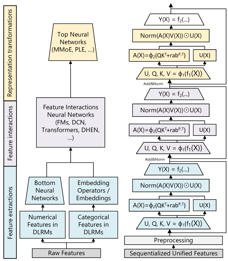 Figure 3 (Zhai et al., 2024): Architecture comparison of traditional DLRMs (left) vs. Generative Recommenders using HSTU (right). The HSTU block replaces the Transformer block with three sequential sub-layers: (1) a pointwise SiLU projection expanding to \(U, V, Q, K\); (2) spatial aggregation via \(\varphi_2(QK^\top + \text{rab}) V\) without softmax normalization; and (3) a pointwise transformation gating the aggregated values by \(U\).
3.4 Why Pointwise Attention Instead of Softmax
The key departure is replacing softmax with SiLU. This is motivated by a formal argument about non-stationary vocabularies.
Softmax normalization forces: \(\sum_j \alpha_{ij} = 1\) for each query \(i\). This normalizes away the magnitude of preference signals. If a user strongly prefers item \(j\), the attention weight \(\alpha_{ij}\) is high relative to others — but the absolute magnitude \(q_i^\top k_j\) is lost in the normalization.
The non-stationarity problem: In recommendation, user preferences are non-stationary — the set of relevant items and actions changes over time. Under a Dirichlet Process model of item popularity (a realistic model for streaming recommendation data), the authors show that softmax attention is suboptimal because it cannot distinguish how strongly the user prefers an item — only relatively among the current candidate set.
Empirical validation (Table 1 on synthetic Dirichlet Process data):
| Variant | HR@10 | HR@50 |
|---|---|---|
| Standard Transformer (softmax) | 0.0442 | 0.2025 |
| HSTU (no rab, softmax) | 0.0617 | 0.2496 |
| HSTU (no rab, pointwise SiLU) | 0.0893 | 0.3170 |
The gap between softmax and pointwise HSTU is 44.7% relative on HR@10 — a dramatic validation of the theoretical argument.
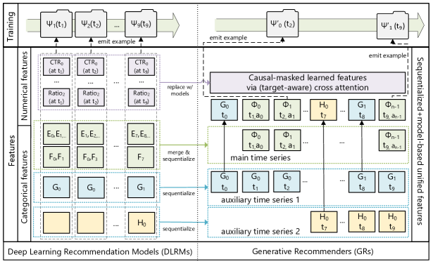 Figure 2 (Zhai et al., 2024): The paradigm shift from DLRMs to Generative Recommenders. DLRMs (left) require separate feature engineering for numerical and categorical features, impression-level training, and distinct retrieval/ranking pipelines. HSTU-based GRs (right) consume raw categorical sequences in a single forward pass, using a unified generative objective that simultaneously trains retrieval and ranking.
3.5 Temporal Relative Attention Bias
The term \(\text{rab}^{p,t}\) adds a learned bias to each attention score based on the relative position and relative time between positions \(i\) and \(j\):
\[\text{rab}^{p,t}_{ij} = b^p_{|i-j|} + b^t_{\lfloor \log_2(\Delta t_{ij}) \rfloor}\]
where \(\Delta t_{ij}\) is the elapsed time (in seconds) between events \(i\) and \(j\), log-bucketed. This encodes two inductive biases: - Positional locality: recent interactions are more relevant (captured by position offset \(|i-j|\)). - Temporal recency: items interacted with recently (small \(\Delta t\)) are more relevant (log-scale bucketing covers seconds to months).
Motivation: Absolute positional encodings (sinusoidal or learned) assume a fixed sequence structure, which is violated when sequence lengths vary by orders of magnitude (some users have 10 interactions, others have 100,000). Relative biases are invariant to absolute position and generalize across sequence lengths.
4. Computational Efficiency
4.1 Generative Training vs. Impression-Level Training
Where the per-pass cost comes from. An attention-based model processing a sequence of length \(n\) has two dominant operations per layer:
- Self-attention: the query-key product \(QK^\top \in \mathbb{R}^{n \times n}\) requires \(n^2\) dot products, each over a \(d\)-dimensional vector — cost \(O(n^2 d)\).
- Feed-forward: a position-wise MLP with hidden dimension \(d_{\text{ff}}\) applies an \(O(d_{\text{ff}} d)\) operation at each of the \(n\) positions — cost \(O(n d_{\text{ff}} d)\).
A single forward pass over a sequence of length \(n_i\) therefore costs \(O(n_i^2 d + n_i d_{\text{ff}} d)\).
Impression-level training. In DLRM-style training, each user contributes \(n_i\) independent training examples — one per logged impression. Each example is a tuple \((\text{user features},\ x_t,\ y_t)\) where \(x_t\) is the item shown in that impression and \(y_t \in \{0,1\}\) is whether the user clicked. The model takes the user’s compressed representation (built from history aggregates and engineered features) together with \(x_t\)’s features and predicts \(p(\text{click} \mid u, x_t)\). Each example is processed as a fully independent forward pass — there is no mechanism to share computation across the \(n_i\) examples belonging to the same user. To train on all \(n_i\) impressions for user \(i\), the model runs \(n_i\) separate forward passes:
\[\text{Cost}_i^{\text{impression}} = n_i \cdot \underbrace{\left(n_i^2 d + n_i d_{\text{ff}} d\right)}_{\text{one forward pass of length } n_i}\]
Summing over users and bounding by the worst case \(N = \max_i n_i\):
\[\sum_i \text{Cost}_i^{\text{impression}} = O(N^3 d + N^2 d_{\text{ff}} d)\]
Why \(n_i\) separate passes? Because impression-level training processes each (user, candidate) pair as a self-contained example — there is no mechanism to share computation across the \(n_i\) targets of the same user. Each pass encodes the full user history into a fixed-length vector and scores one target against it.
Generative training. The generative approach replaces \(n_i\) separate passes with a single teacher-forced forward pass under a causal mask. Concretely:
- The full sequence \((x_0, x_1, \ldots, x_{n_i - 1})\) is fed into the model at once.
- A causal mask enforces that position \(t\) can only attend to positions \(0, \ldots, t-1\) — the model never sees the future within the same pass.
- The output at position \(t\) is a prediction of \(x_{t+1}\), using only the causal prefix.
One forward pass at cost \(O(n_i^2 d + n_i d_{\text{ff}} d)\) therefore produces all \(n_i\) predictions simultaneously. The causal mask makes this informationally equivalent to running \(n_i\) separate prefix-conditioned passes — but shares the \(O(n_i^2 d)\) attention computation across all predictions rather than repeating it \(n_i\) times.
The role of \(s_u(n_i)\). Even though the generative forward pass produces \(n_i\) predictions, you don’t necessarily compute the loss — and backpropagate gradients — for all of them. The scalar \(s_u(n_i) \in (0, 1]\) is the fraction of positions sampled as loss targets in a given training step.
Two reasons to set \(s_u < 1\):
- Gradient normalization. A user with \(n_i = 10{,}000\) interactions would contribute 1,000× more gradient signal than a user with \(n_i = 10\) if all positions were used. Setting \(s_u(n_i) = c / n_i\) for a constant \(c\) equalizes each user’s contribution regardless of sequence length.
- Output projection cost. Predicting the next item requires projecting the hidden state \(u_t \in \mathbb{R}^d\) into the item embedding space — a cost of \(O(d^2)\) or \(O(d \cdot |\mathcal{V}|)\) per position. For large item vocabularies, this per-position output cost dominates if all \(n_i\) positions are used.
The key point is that \(s_u\) does not affect the attention computation. The \(O(n_i^2 d)\) forward pass is incurred once regardless of how many targets are sampled — you cannot avoid attending over the full sequence just because you only want one prediction. \(s_u\) only controls how many output projections and loss evaluations follow the shared forward pass.
Example. Say user \(i\) has history \((x_0, x_1, x_2, x_3, x_4)\). One causal forward pass produces hidden states at every position:
\[\underbrace{x_0 \to u_0,\quad x_1 \to u_1,\quad x_2 \to u_2,\quad x_3 \to u_3,\quad x_4 \to u_4}_{\text{one forward pass, cost } O(n_i^2 d)}\]
where \(u_t\) is conditioned on \((x_0, \ldots, x_t)\) only (enforced by the causal mask). Each \(u_t\) can predict the next item \(x_{t+1}\), giving four candidate loss targets:
| Position \(t\) | Prediction | Ground truth | Compute loss? |
|---|---|---|---|
| 0 | \(\text{proj}(u_0) \approx x_1\) | \(x_1\) | maybe |
| 1 | \(\text{proj}(u_1) \approx x_2\) | \(x_2\) | maybe |
| 2 | \(\text{proj}(u_2) \approx x_3\) | \(x_3\) | maybe |
| 3 | \(\text{proj}(u_3) \approx x_4\) | \(x_4\) | maybe |
With \(s_u = 1/n_i = 1/5\), one position is sampled at random — say \(t = 2\). Only \(-\log p(x_3 \mid u_2)\) is evaluated; the hidden states at positions 0, 1, 3 are computed but discarded. The \(O(n_i^2 d)\) attention cost was already paid for all of them.
Setting \(s_u(n_i) = 1/n_i\) (one target per user per step), the total cost per user is:
\[\text{Cost}_i^{\text{generative}} = \underbrace{n_i^2 d + n_i d_{\text{ff}} d}_{\text{forward pass (fixed)}} + \underbrace{\frac{1}{n_i} \cdot n_i \cdot d^2}_{s_u \cdot n_i \text{ output projections}} = n_i^2 d + n_i d_{\text{ff}} d + d^2\]
Dropping the \(d^2\) term (dominated for large \(n_i\)) and summing over users:
\[\sum_i \text{Cost}_i^{\text{generative}} = O(N^2 d + N d_{\text{ff}} d)\]
This is an \(O(N)\) reduction relative to impression-level training. A user with 1,000 interactions costs \(O(N^2 d)\) rather than \(O(N^3 d)\), simply because the forward pass is shared across all their predictions instead of repeated for each one.
4.2 Stochastic Length Sparsity
Long sequences (power-law distributed in real recommendation data) dominate attention cost. HSTU handles them via stochastic length (SL) truncation. Let \(N^\alpha\) be a target complexity budget with \(\alpha \in (1, 2]\). For user \(i\) with sequence length \(n_i\):
\[\text{SL}(n_i, N^{\alpha/2}) = \begin{cases} (x_0, \ldots, x_{n_i-1}) & \text{if } n_i \leq N^{\alpha/2} \\ \Gamma(n_i, N^{\alpha/2}) & \text{if } n_i > N^{\alpha/2},\ \text{with probability } 1 - N^\alpha / n_i^2 \\ (x_0, \ldots, x_{n_i-1}) & \text{if } n_i > N^{\alpha/2},\ \text{with probability } N^\alpha / n_i^2 \end{cases}\]
where \(\Gamma(n_i, N^{\alpha/2})\) denotes random subsampling to length \(N^{\alpha/2}\).
The expected attention cost per user becomes \(O(N^\alpha d)\). With \(\alpha < 2\), this is subquadratic. For \(\alpha = 1.5\), for example, a sequence of length \(10^6\) has effective cost \(O(10^9)\) instead of \(O(10^{12})\).
Empirically, this achieves 80%+ sparsity on long-tail users with less than 0.2% metric degradation.
4.3 M-FALCON: Inference Amortization
At inference time, ranking requires scoring \(b_m\) candidate items. Naively, each candidate requires a separate forward pass: cost \(O(b_m \cdot n^2 d)\).
M-FALCON (Microbatch FALCON) processes \(b_m\) candidates simultaneously by modifying attention masks so that candidate items attend to user history but not to each other:
- User history of length \(n\) is computed once: cost \(O(n^2 d)\).
- Each candidate \(x_c\) attends to the history via cross-attention: cost \(O(n d)\) per candidate.
- Total: \(O(n^2 d + b_m n d)\) — amortized to effectively \(O(n^2 d)\) when \(b_m \ll n\).
The relative attention bias \(\text{rab}^{p,t}\) is modified to place candidates at a consistent temporal position relative to the user history, enabling consistent attention patterns across the microbatch.
This achieves 5.6× inference speedup and allows a 285× model complexity increase while maintaining 1.5–2.5× throughput improvements in production.
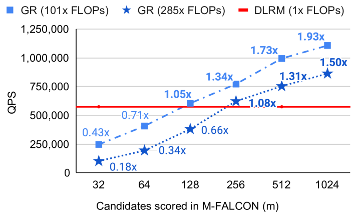 Figure 7 (Zhai et al., 2024): M-FALCON inference throughput. By processing \(b_m\) candidate items simultaneously via modified attention masks (candidates attend to history but not each other), GR at 285× model complexity achieves 1.3–1.9× the throughput of the DLRM baseline (red line) for microbatch sizes \(m \geq 256\). The amortization effect is visible as QPS rises with larger \(m\).
4.4 Memory Efficiency vs. Standard Transformers
Standard Transformer blocks have per-layer activation memory proportional to \(33d\) (in bfloat16). HSTU reduces this to \(14d\) through:
- Eliminating the softmax normalization step (saves the \(n \times n\) softmax matrix).
- Fusing the SiLU nonlinearity into the projection.
- The gated structure removes the need for a separate feed-forward sublayer.
Result: HSTU can stack 2× deeper networks for the same GPU memory budget, contributing directly to the scaling law results.
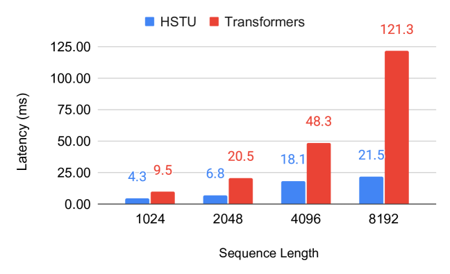 Figure 6 (Zhai et al., 2024): Training latency comparison between HSTU and standard Transformers across sequence lengths. HSTU’s subquadratic attention (via stochastic length sparsity and fused raggified attention) scales substantially better: at sequence length 8,192, HSTU achieves 21.5ms latency vs. 121.3ms for a standard Transformer — a 5.6× speedup.
5. Scaling Laws
HSTU demonstrates power-law scaling across three orders of magnitude in training compute, matching the scaling behavior of GPT-3 and LLaMA-2:
\[\text{HR@100} \propto C^\beta \quad \text{for } C \in [10^{20},\ 10^{23}] \text{ FLOPs}\]
where the exponent \(\beta\) is empirically fitted from Figure 7. The paper does not state the exact value of \(\beta\), but the log-log plot shows a clean linear fit — characteristic of a true power law.
Key observations:
- DLRMs plateau around 200B parameters; HSTU continues scaling to 1.5 trillion parameters.
- The scaling behavior holds for both retrieval (HR@100) and ranking (NE) metrics.
- The scaling curve matches the training-compute curves of GPT-3/LLaMA-2 when plotted on the same axes.
Why does HSTU scale while DLRMs do not?
DLRMs use impression-level scoring, which fundamentally limits data efficiency: each training example provides exactly one bit of supervision (click or no-click) for one (user, item) pair. As the model grows, the training signal per parameter decreases faster than for sequence models, leading to early saturation.
HSTU’s generative training extracts \(n_i\) supervised signals per user sequence: each position predicts the next item. For a user with 1,000 interactions, this is a 1,000× improvement in supervision density per forward pass. More parameters can be productively trained because the signal-to-parameter ratio remains favorable.
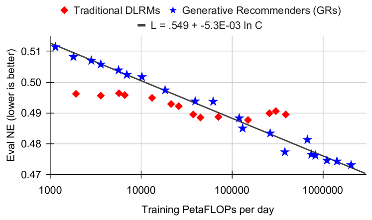 Figure 7c (Zhai et al., 2024): Ranking scaling law (NE metric). GRs follow a clean log-linear scaling law \(L = 0.549 - 5.3 \times 10^{-3} \ln C\) across three orders of magnitude in training compute (\(10^3\) to \(10^6\) PetaFLOPs/day), while traditional DLRMs plateau and fail to improve beyond a compute threshold. This is the recommendation-domain analogue of the Chinchilla scaling law.
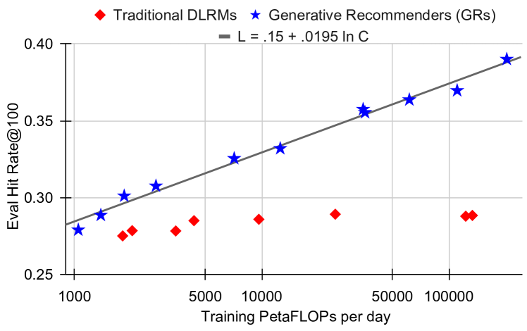 Figure 7a (Zhai et al., 2024): Retrieval scaling law (HR@100 metric). GRs scale continuously with compute — fit \(\text{HR@100} = 0.15 + 0.0195 \ln C\) — while DLRMs (red) cluster around HR@100 ≈ 0.28–0.29 regardless of compute budget, confirming the plateau is architectural rather than fundamental.
6. Experiments
6.1 Synthetic Validation: Dirichlet Process Data
To isolate architectural effects from data-specific factors, the authors generate synthetic data from a Dirichlet Process (DP) model of user preferences: - Items are drawn from a DP with concentration \(\theta\): popular items receive exponentially more weight. - Each user has a hidden preference distribution; their history is sampled from it.
| Architecture | HR@10 | HR@50 |
|---|---|---|
| Standard Transformer | 0.0442 | 0.2025 |
| HSTU (no rab, softmax) | 0.0617 | 0.2496 |
| HSTU (no rab, pointwise) | 0.0893 | 0.3170 |
| HSTU (full) | best | best |
The 44.7% gap between softmax and pointwise (no rab, same architecture otherwise) directly validates the theory about preference intensity and non-stationarity.
6.2 Public Benchmarks
On MovieLens-1M:
| Method | HR@10 | NDCG@10 |
|---|---|---|
| SASRec | 0.2828 | 0.1545 |
| BERT4Rec | 0.2701 | 0.1445 |
| HSTU (base) | 0.3043 (+7.6%) | 0.1700 (+10.1%) |
| HSTU-large | 0.3306 (+16.9%) | 0.1858 (+20.3%) |
On Amazon Books (HR@10):
| Method | HR@10 | NDCG@10 |
|---|---|---|
| SASRec | baseline | baseline |
| HSTU-large | +60.6% relative | +65.8% relative |
6.3 Industrial Streaming Data
Standard Transformers produce NaN loss on industrial streaming data with long-tail sequence lengths and non-stationary vocabulary. HSTU trains stably on sequences of length up to 8,192 with the following efficiency:
- Training throughput: 5.3–15.2× faster than FlashAttention2-based Transformers.
- Memory bandwidth: \(O(\sum_i n_i^2 d_{qk}^2 R^{-1})\) through raggified attention fusion (R = reuse factor).
6.4 Online A/B Tests
Deployed as GR (Generative Recommender) at Meta scale (billions of users), validated via A/B testing:
| System | Metric | Improvement |
|---|---|---|
| GR Ranking | Engagement (online A/B) | +12.4% |
| GR Retrieval | HR@100 | +5.1% |
| GR Retrieval | HR@500 | +1.9% |
| GR Retrieval | Engagement | +6.2% |
| GR Retrieval | Consumption | +5.0% |
These are among the largest reported recommendation system improvements in recent literature.
7. Relation to Wukong
See Wukong for the companion paper. Despite appearing in the same month and addressing the same fundamental gap (no scaling law for recommendation systems), Wukong and HSTU are structurally very different:
| Aspect | Wukong | HSTU |
|---|---|---|
| Problem framing | CTR prediction over dense feature sets | Sequential transduction over user behavior history |
| Core operation | Factorization Machine (pairwise dot products) | Attention (query-key matching) |
| Data representation | Feature matrix \(X \in \mathbb{R}^{n \times d}\) (one row per feature) | Time series \(h \in \mathbb{R}^{T \times d}\) (one row per event) |
| Interaction mechanism | Explicit: \(XX^\top Y\) generates controlled cross-feature products | Implicit: \(QK^\top\) generates attention-weighted history aggregation |
| Scaling driver | Depth → exponential interaction order (\(2^l\) after \(l\) layers) | Scale → more parameters efficiently trained via generative supervision |
| Submission date | March 4, 2024 | February 26, 2024 |
| Team | Meta Ads (same team as DHEN) | Meta AI Research |
The logical connection. Both papers are best understood as responses to the same empirical observation: DLRM-style models plateau while LLMs scale. Wukong’s response is within the DLRM paradigm: fix the interaction module so that expressivity grows with depth. HSTU’s response is across paradigms: abandon the DLRM framing entirely and treat recommendation as a generative sequential problem.
Neither paper is a strict continuation of the other (HSTU was submitted first). Rather, they are parallel evidence for the same thesis: the recommendation scaling barrier is architectural, not fundamental. Together they triangulate the space of solutions — one extending the feature-interaction approach to its principled limit, the other importing the full generative modeling paradigm from NLP.
A unified future architecture would likely combine: - Wukong’s principled feature interaction (FM stack) for structured contextual features - HSTU’s sequential modeling and generative training for user history sequences
8. References
| Reference Name | Brief Summary | Link |
|---|---|---|
| Actions Speak Louder than Words: Trillion-Parameter Sequential Transducers | Main HSTU paper | https://arxiv.org/abs/2402.17152 |
| Wukong: Towards a Scaling Law for Large-Scale Recommendation | Companion paper; FM-stack approach | https://arxiv.org/abs/2403.02545 |
| SASRec: Self-Attentive Sequential Recommendation | Key sequential recommendation baseline | https://arxiv.org/abs/1808.09781 |
| BERT4Rec: Sequential Recommendation with BERT | BERT-based sequential baseline | https://arxiv.org/abs/1904.06690 |
| Scaling Laws for Neural Language Models (Kaplan et al.) | Original power-law scaling for LLMs | https://arxiv.org/abs/2001.08361 |
| FlashAttention-2: Faster Attention with Better Parallelism | Efficient attention baseline for speed comparison | https://arxiv.org/abs/2307.08691 |
| DLRM: An Advanced, Open Source Deep Learning Recommendation Model | Meta DLRM baseline that plateaus | https://arxiv.org/abs/1906.00091 |
| Deep Interest Network for Click-Through Rate Prediction (Zhou et al., KDD 2018) | Introduces target-aware local activation: candidate-conditioned attention over user history where weights are derived from the outer product of history and candidate embeddings (no softmax normalization). Foundational justification for removing handcrafted numerical features in HSTU — target-aware attention implicitly recomputes what static aggregates approximate, conditioned on each candidate. | https://arxiv.org/abs/1706.06978 |
| Breaking the Curse of Quality Saturation with User-Centric Ranking (Zhao et al., KDD 2023) | Formal analysis and empirical evidence that item-centric DLRMs hit a hard asymptotic error floor as item inventory grows; motivates HSTU’s abandonment of per-item embeddings | https://arxiv.org/abs/2305.15333 |
| SiLU / Swish Activation: Gaussian Error Linear Units | Theoretical basis for SiLU nonlinearity | https://arxiv.org/abs/1606.08415 |
| Dirichlet Process Mixture Models | Statistical model motivating pointwise attention design | https://www.gatsby.ucl.ac.uk/~ywteh/research/npbayes/dpchp.pdf |