QJL: 1-Bit Quantized JL Transform for KV Cache Quantization with Zero Overhead
Amir Zandieh, Majid Daliri, Insu Han — arXiv:2406.03482 [cs.LG], July 2024
| Dimension | Prior State | This Paper | Key Result |
|---|---|---|---|
| Quantization overhead | Methods store a zero-point + scale per block, adding ~1–2 extra bits per quantized number | JL transform + sign-bit: no stored normalization constants | Zero memory overhead |
| Inner product estimator | Symmetric sign-bit estimator estimates angle, not inner product (biased) | Asymmetric: quantize only the key; leave the query unquantized | Unbiased with same distortion guarantee as standard JL |
| Compression ratio | KIVI / KVQuant at 3–4.3 bits with overhead | 3 bits effective per FPN | >5× reduction vs. FP16 baseline |
| Attention accuracy | — | Theorem 3.6: relative error ≤ 3ε on all attention scores simultaneously | \(m = O(\varepsilon^{-2} \log n)\) bits per token, independent of embedding dimension \(d\) |
Relations
Builds on: TurboQuant (see also; QJL is the primitive used there) Extended by: PolarQuant, TurboQuant Concepts used: JL Transform and Metric Dimension Reduction
Table of Contents
- 1. The KV Cache Overhead Problem
- 2. The QJL Transform
- 3. Attention Score Approximation
- 4. Algorithm and Implementation
- 5. Experiments
- 6. References
1. The KV Cache Overhead Problem
📐 In autoregressive transformer decoding, the attention output at step \(n\) is
\[o_n = \sum_{i \in [n]} \text{Score}(i) \cdot v_i, \qquad \text{Score} := \text{softmax}\bigl([\langle q_n, k_1\rangle, \ldots, \langle q_n, k_n\rangle]\bigr).\]
To avoid recomputing all keys and values from scratch, the model caches \(\{k_i, v_i\}_{i \in [n]}\) — the KV cache. For long contexts this cache dominates GPU memory.
The natural fix is quantization: store each FP16/BF16 number in fewer bits. But every existing method (KIVI, KVQuant, etc.) groups coordinates into blocks and stores a zero point and scale per block. Depending on block size, this metadata adds ≈1–2 extra bits per quantized value, nearly doubling the apparent saving.
Classical uniform quantizers map \([x_{\min}, x_{\max}]\) to \(\{0, 1, \ldots, 2^b - 1\}\). To dequantize you need \(x_{\min}\) and the step size \(\Delta = (x_{\max} - x_{\min})/2^b\). Storing these two FP16 numbers per block of \(G\) coordinates adds \(32/G\) bits per coordinate. For \(G = 16\), this is \(+2\) bits — a major fraction of a 3-bit quantizer.
A \(b\)-bit uniform quantizer maps a scalar \(x \in [x_{\min}, x_{\max}]\) to one of \(2^b\) equally-spaced levels \(\{0, 1, \ldots, 2^b - 1\}\) via \[\hat{x} = \left\lfloor \frac{x - x_{\min}}{\Delta} \right\rfloor, \qquad \Delta = \frac{x_{\max} - x_{\min}}{2^b - 1}.\] For \(b = 3\) there are 8 levels; each value is stored in 3 bits. Dequantization recovers \(x \approx x_{\min} + \hat{x}\cdot\Delta\), which requires \(x_{\min}\) and \(\Delta\) (or equivalently a zero-point and scale). These constants must be stored alongside the quantized values — the source of the overhead described above.
QJL sidesteps metadata entirely by replacing the classical quantizer with a sketching operation whose output distribution is analytically known from the design of the sketch.
A sketch (or linear sketch) of a vector \(x \in \mathbb{R}^d\) is a compressed representation \(Sx \in \mathbb{R}^m\) produced by a random linear map \(S \in \mathbb{R}^{m \times d}\) with \(m \ll d\). The sketching operation is the act of applying \(S\). Unlike classical quantization, the output distribution of \(Sx\) is determined entirely by the distribution of \(S\) — no per-vector calibration constants (zero-point, scale) are needed to interpret the result. The Johnson–Lindenstrauss transform is a canonical sketch: for \(S_{ij} \overset{\text{i.i.d.}}{\sim} \mathcal{N}(0,1)\), the rescaled sketch \(\frac{1}{\sqrt{m}}Sx\) preserves \(\ell_2\) norms and pairwise inner products up to \((1\pm\varepsilon)\) with high probability. QJL goes one step further by sign-quantizing the sketch output (\(\operatorname{sign}(Sk) \in \{-1,+1\}^m\)), reducing storage to 1 bit per sketch coordinate.
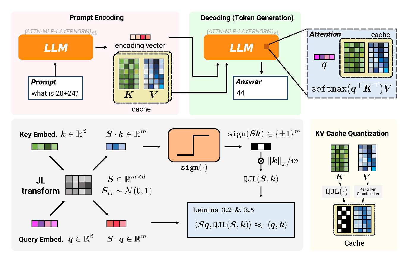 Figure 1 (Zandieh et al., 2024): The QJL pipeline. During prompt encoding (left), key embeddings are projected via a random JL matrix S, sign-quantized to 1 bit, and cached together with the scalar norm. During token generation (right), the query is projected by the same S and its inner product with each cached sign vector is computed, yielding an unbiased estimate of the full-precision attention score — with no stored quantization constants.
2. The QJL Transform
Let \(S \in \mathbb{R}^{m \times d}\) have i.i.d. entries \(S_{ij} \sim \mathcal{N}(0,1)\). For any \(q, k \in \mathbb{R}^d\), the standard JL estimator of \(\langle q, k\rangle\) is \[\operatorname{ProdJL}(q,k) := \frac{1}{m}\langle Sq, Sk\rangle.\] Unbiasedness: \(\mathbb{E}_S[\operatorname{ProdJL}(q,k)] = \langle q,k\rangle\), since \(\mathbb{E}[S^\top S] = I_d\).
Distortion guarantee: For \(m = O(\varepsilon^{-2}\log(1/\delta))\), \[\Pr_S\!\bigl[|\operatorname{ProdJL}(q,k) - \langle q,k\rangle| > \varepsilon\|q\|_2\|k\|_2\bigr] \leq \delta.\]
Storage cost: Caching \(Sk\) requires \(m\) full-precision floats (16 bits each), for a total of \(16m\) bits per key token. QJL replaces \(Sk\) with \(\operatorname{sign}(Sk) \in \{-1,+1\}^m\) (1 bit each) plus one scalar \(\|k\|_2\) (16 bits) — a \(16\times\) reduction in sketch storage at the cost of a modest increase in the distortion constant.
Why not skip the JL step entirely (“QL”)? A natural cheaper alternative is to sign-quantize \(k\) directly in \(\mathbb{R}^d\) — call this QL: \[\widehat{\langle q,k\rangle}_{\text{QL}} := c \cdot \|k\|_2 \cdot \langle q, \operatorname{sign}(k)\rangle.\] This fails for three reasons.
1. No statistical structure to analyze. With QL, \(\operatorname{sign}(k)\) is a deterministic function of \(k\) — there is no random variable to average over. The error \(\langle q,k\rangle - c\|k\|_2\langle q,\operatorname{sign}(k)\rangle\) is a single fixed number that can be arbitrarily large; “unbiasedness” is not even a meaningful statement.
2. The unbiasedness proof requires Gaussian independence. The key step in proving \(\mathbb{E}_S[\operatorname{ProdQJL}] = \langle q,k\rangle\) is decomposing \(q = \frac{\langle q,k\rangle}{\|k\|_2^2}k + q^{\perp k}\) and showing the cross term vanishes: \[\mathbb{E}\bigl[s_i^\top q^{\perp k} \cdot \operatorname{sign}(s_i^\top k)\bigr] = 0.\] This uses the fact that \(s_i^\top k\) and \(s_i^\top q^{\perp k}\) are independent — they are uncorrelated Gaussians (since \(k \perp q^{\perp k}\)), and joint Gaussianity of \((s_i^\top k,\, s_i^\top q^{\perp k})\) promotes uncorrelatedness to independence. For QL the analogous term is \(q_i^{\perp k}\cdot\operatorname{sign}(k_i)\): there is no joint Gaussianity, independence fails, and the cross term does not vanish.
3. Sign quantization is extremely lossy for skewed vectors. Key vectors in transformers have outlier coordinates — a few large-magnitude dimensions and many near-zero ones (empirically visible in the key cache outlier plots). Direct sign quantization assigns equal weight \(\pm 1\) to every coordinate regardless of magnitude, so the estimate is dominated by the signs of the outlier dimensions irrespective of \(q\). The JL projection fixes this by isotropizing \(k\): each projected coordinate \(s_i^\top k \sim \mathcal{N}(0,\|k\|_2^2)\) has the same distribution for any \(k\), making sign quantization uniformly efficient across all key vectors.
2.1 Definition
🔑 Definition (QJL and inner product estimator). For positive integers \(d, m\), let \(S \in \mathbb{R}^{m \times d}\) be a JL matrix with i.i.d. entries \(S_{ij} \sim \mathcal{N}(0, 1)\). The Quantized JL (QJL) transform is
\[H_S(k) := \operatorname{sign}(Sk) \in \{-1, +1\}^m.\]
For any pair \(q, k \in \mathbb{R}^d\), the asymmetric inner product estimator is
\[\operatorname{ProdQJL}(q, k) := \frac{\sqrt{\pi/2}}{m} \cdot \|k\|_2 \cdot \langle Sq,\; H_S(k)\rangle.\]
If we applied QJL to both vectors we would obtain an unbiased estimator of the angle \(\theta(q,k)\), not the inner product \(\langle q, k\rangle = \|q\|\|k\|\cos\theta\). Recovering the cosine from the angle estimate via \(\cos(\hat\theta)\) introduces bias. The fix: quantize only \(k\) (the cached vector), leave \(q\) (the fresh query vector, already in memory) unquantized.
Yes — during inference, each key token \(k_i\) is never stored directly. Instead the cache holds \(H_S(k_i) = \operatorname{sign}(Sk_i) \in \{-1,+1\}^m\) (\(m\) bits) and the scalar \(\|k_i\|_2\) (1 FP16 = 16 bits), totalling \(m + 16\) bits per token. The original key required \(16d\) bits (FP16). So the compression ratio is \[\frac{16d}{m + 16}.\] The 16× figure refers specifically to the sketch storage (\(Sk\) at FP16 → \(\operatorname{sign}(Sk)\) at 1 bit/coord), not the overall ratio. The overall key cache compression depends on how \(m\) is chosen relative to \(d\): with \(d = 256\) and \(m \approx 750\) bits (sufficient for 32k-token contexts at \(\varepsilon = 0.2\)), the ratio is roughly \(\frac{16 \times 256}{750 + 16} \approx 5.3\times\) — matching the paper’s reported “>5× vs. FP16 baseline”. The value cache is separate and unaffected by QJL. The query \(q_n\) is never cached at all (it is always fresh at each decode step).
2.2 Unbiasedness (Lemma 3.2)
Lemma (Inner product estimator ProdQJL is unbiased). For any \(q, k \in \mathbb{R}^d\),
\[\mathbb{E}_S[\operatorname{ProdQJL}(q, k)] = \langle q, k\rangle.\]
📐 Proof sketch. Decompose \(q = \frac{\langle q,k\rangle}{\|k\|_2^2} k + q^{\perp k}\) where \(\langle q^{\perp k}, k\rangle = 0\). Then
\[\operatorname{ProdQJL}(q,k) = \frac{\sqrt{\pi/2}}{m} \sum_{i \in [m]} \Bigl[\frac{\langle q,k\rangle}{\|k\|_2} |s_i^\top k| + \|k\|_2 \cdot s_i^\top q^{\perp k} \cdot \operatorname{sign}(s_i^\top k)\Bigr].\]
Each \(s_i\) is a standard Gaussian row. Because \(k \perp q^{\perp k}\), the projections \(s_i^\top k\) and \(s_i^\top q^{\perp k}\) are independent Gaussians (Fact: jointly Gaussian, uncorrelated ⟹ independent). Therefore the cross term vanishes: \(\mathbb{E}[s_i^\top q^{\perp k} \cdot \operatorname{sign}(s_i^\top k)] = 0\).
For the first term, \(x := s_i^\top k \sim \mathcal{N}(0, \|k\|_2^2)\), so \(\mathbb{E}[|x|] = \sqrt{2/\pi}\,\|k\|_2\) by the half-normal formula. Substituting:
\[\mathbb{E}[\operatorname{ProdQJL}(q,k)] = \sqrt{\pi/2} \cdot \frac{\langle q,k\rangle}{\|k\|_2} \cdot \sqrt{2/\pi}\,\|k\|_2 = \langle q,k\rangle. \quad \square\]
If \(X \sim \mathcal{N}(0, \sigma^2)\), then \(\mathbb{E}[|X|] = \sigma\sqrt{2/\pi}\). Derivation: by symmetry, \[\mathbb{E}[|X|] = 2\int_0^\infty x \cdot \frac{1}{\sigma\sqrt{2\pi}}\,e^{-x^2/(2\sigma^2)}\,dx.\] Substitute \(u = x^2/(2\sigma^2)\), so \(x\,dx = \sigma^2\,du\): \[= \frac{2}{\sigma\sqrt{2\pi}}\int_0^\infty e^{-u}\,\sigma^2\,du = \frac{2\sigma}{\sqrt{2\pi}}\cdot 1 = \sigma\sqrt{\tfrac{2}{\pi}}.\] In context, \(x = s_i^\top k \sim \mathcal{N}(0,\|k\|_2^2)\), so \(\sigma = \|k\|_2\) and \(\mathbb{E}[|s_i^\top k|] = \|k\|_2\sqrt{2/\pi}\).
The standard JL estimator \(\frac{1}{m}\langle Sq, Sk\rangle\) is also unbiased for \(\langle q,k\rangle\) (the JL lemma). QJL replaces \(Sk \in \mathbb{R}^m\) (32 bits per entry) with \(\operatorname{sign}(Sk) \in \{-1,+1\}^m\) (1 bit per entry), at the cost of one stored scalar \(\|k\|_2\) (FP16). The \(\sqrt{\pi/2}\) prefactor corrects for the sign-collapse that shrinks the expected magnitude.
2.3 Distortion Bound (Lemma 3.5)
Lemma (Distortion of ProdQJL). For any \(q, k \in \mathbb{R}^d\), if \(m \geq \frac{4}{3} \cdot \frac{1+\varepsilon}{\varepsilon^2} \log\frac{2}{\delta}\), then
\[\Pr_S\!\bigl[|\operatorname{ProdQJL}(q,k) - \langle q,k\rangle| > \varepsilon\|q\|_2\|k\|_2\bigr] \leq \delta.\]
Proof sketch. Each term \(z_i := \sqrt{\pi/2}\,\|k\|_2 \cdot s_i^\top q \cdot \operatorname{sign}(s_i^\top k)\) is i.i.d. with \(\mathbb{E}[z_i] = \langle q,k\rangle/m\) (by unbiasedness). Its \(\ell\)-th moment obeys \(\mathbb{E}[|z_i|^\ell] = (\pi/2)^{\ell/2} \|k\|_2^\ell \mathbb{E}[|s_i^\top q|^\ell]\). Because \(s_i^\top q \sim \mathcal{N}(0, \|q\|_2^2)\), the moments are \(\sigma^\ell \cdot 2^{\ell/2}\Gamma((\ell+1)/2)/\sqrt{\pi}\). A Bernstein inequality applied to the mean \(\frac{1}{m}\sum z_i\) gives the stated tail bound. Notably, the constants are smaller than those for the unquantized JL estimator.
3. Attention Score Approximation
🔑 Theorem 3.6 (Distortion bound on QJL key cache quantizer). Suppose all key and query embeddings have bounded norm \(\max_i \|k_i\|_2, \|q_n\|_2 \leq r\). If \(m \geq 2r^2\varepsilon^{-2}\log n\), then with probability \(1 - 1/\text{poly}(n)\), simultaneously for all \(i \in [n]\):
\[|\widehat{\text{Score}}(i) - \text{Score}(i)| \leq 3\varepsilon \cdot \text{Score}(i).\]
Proof sketch. By Lemma 3.5 with union bound over \(n\) token pairs, all estimated inner products \(\widehat{qK}(j)\) satisfy \(|\widehat{qK}(j) - \langle q_n, k_j\rangle| \leq \varepsilon\) simultaneously with high probability. Applying the softmax map turns additive errors into \((1 \pm 3\varepsilon)\) multiplicative errors on the scores.
The key insight: only \(m = O(\varepsilon^{-2}\log n)\) sign bits per token are needed, regardless of the embedding dimension \(d\). In practice, with \(n = 32{,}000\) tokens and \(\varepsilon = 0.2\), this means \(m \approx 750\) bits per key — about 3 bits/coordinate for \(d = 256\).
4. Algorithm and Implementation
4.1 Key Cache Quantization Algorithm
# QJL Key Cache Quantizer
def setup(d, m):
    S = np.random.randn(m, d)          # JL matrix, i.i.d. N(0,1)
    Q, _ = np.linalg.qr(S.T)          # orthogonalize rows
    S = Q.T[:m]
    return S

def quantize_key(S, k):
    projected = S @ k                  # shape (m,)
    k_tilde = np.sign(projected)       # 1-bit quantization
    nu = np.linalg.norm(k)             # store only the norm
    return k_tilde, nu                 # (m bits) + (1 FP16)

def estimate_scores(S, q, cache):
    Sq = S @ q                         # m-dim vector, computed once
    scores = []
    for k_tilde, nu in cache:
        inner = np.dot(Sq, k_tilde)    # fast int dot product
        est = (np.sqrt(np.pi / 2) / len(k_tilde)) * nu * inner
        scores.append(est)
    return softmax(np.array(scores))
The key cache stores: \(m\) sign bits + 1 FP16 scalar \(\|k\|_2\) per token. Value cache uses standard token-wise quantization (effective and well-studied separately).
4.2 Practical Considerations
Outlier channels. In deeper layers of LLMs like Llama-2, a small number of fixed channels (≈4 out of 128) have much larger magnitudes than the rest. Because Theorem 3.6’s distortion scales as \(r^2\) (the max embedding norm), these outliers disproportionately increase error. Fix: detect outlier channels during the prefill phase and quantize them with a separate, lower-compression QJL instance.
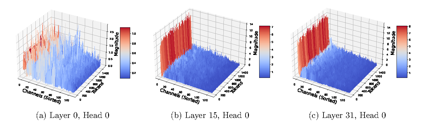 Figure 2 (Zandieh et al., 2024): Key cache entry magnitudes for three representative layers of Llama-2. In the early layer (Layer 0), magnitudes are roughly uniform across channels. By Layer 15 and especially Layer 31, a small number of channels (≈4) exhibit magnitudes orders of magnitude larger than the rest — these are the outlier channels whose large \(r^2\) would inflate QJL’s distortion bound if left unhandled.
Orthogonalizing \(S\). Empirically, QR-decomposing the Gaussian matrix \(S\) (so its rows are orthonormal) almost always improves performance. This is consistent with results on orthogonal random features and super-bit LSH — orthogonality reduces variance.
With i.i.d. Gaussian rows, the dot products \(\{s_i^\top q\}\) are correlated because the rows themselves are correlated (though only weakly, by concentration). Orthogonalized rows make these dot products exactly uncorrelated and suppress variance by the same factor as in orthogonal JL transforms.
5. Experiments
Tested on LongBench (long-range QA) and LM-eval (standard benchmarks) with Llama-2-7B and Llama-3-8B.
| Method | Bits | NarrativeQA | Qasper | HotpotQA | 2WikiMultiQA |
|---|---|---|---|---|---|
| FP16 | 16 | 20.79 | 29.42 | 33.05 | 24.14 |
| KIVI | 3 | 20.96 | 29.01 | 32.79 | 23.01 |
| KVQuant | 4.3 | 20.14 | 28.77 | 34.06 | 23.05 |
| QJL | 3 | 21.83 | 29.44 | 35.62 | 23.60 |
Key result: QJL at 3 bits matches or exceeds FP16 on most tasks, while KIVI/KVQuant degrade. KVQuant is significantly slower during prompting, while QJL matches FP16 decoding speed and reduces memory by >5×.
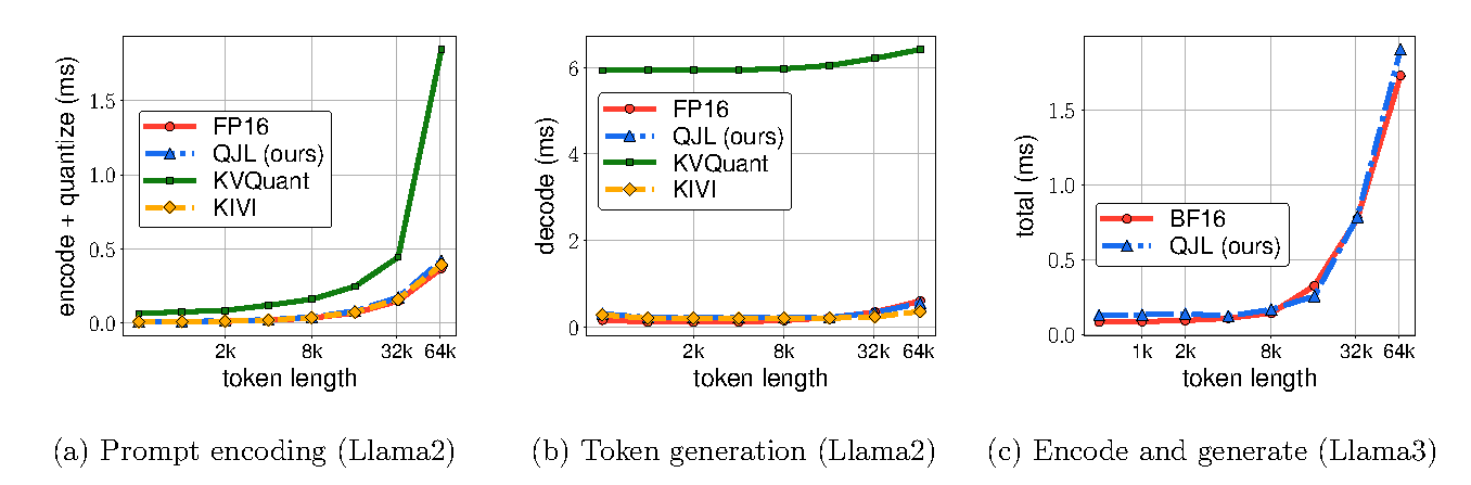 Figure 3 (Zandieh et al., 2024): Wall-clock time (ms) as a function of input sequence length (1k–128k tokens). Left: prompt encoding time — KVQuant is significantly slower due to preprocessing overhead, while QJL and KIVI match FP16. Middle: token generation time — QJL and KIVI are faster than FP16 due to reduced KV cache size; KVQuant is slower. Right: combined encode-and-generate time on Llama3 — QJL achieves at least 5× memory reduction with no runtime overhead.
6. References
| Reference | Brief Summary | Link |
|---|---|---|
| Zandieh et al. (QJL, 2024) | This paper | arXiv:2406.03482 |
| Dasgupta & Gupta (2003) | Elementary proof of JL lemma | Paper |
| Charikar (2002) | SimHash / sign-bit angle estimator | STOC 2002 |
| Liu et al. (KIVI, 2024) | Asymmetric 2-bit KV cache quantization | arXiv:2402.02750 |
| Hooper et al. (KVQuant, 2024) | Per-channel quantization for KV cache | arXiv:2401.18079 |
| Bai et al. (LongBench, 2023) | Long-context bilingual benchmark | arXiv:2308.14508 |