Muon: A Scalable Matrix Orthogonalization Optimizer for LLM Training
Jingyuan Liu, Jianlin Su, et al. (Kimi Team, Moonshot AI) — arXiv 2502.16982, February 2025
| Dimension | Prior State | This Paper | Key Result |
|---|---|---|---|
| Scalability | Original Muon untested beyond small LMs | Weight decay + per-parameter update scaling | Validated on 3B/16B MoE at 5.7T tokens |
| Compute efficiency | AdamW is the de facto standard | Muon under compute-optimal training | ~2x fewer FLOPs to match AdamW loss |
| Theoretical grounding | Heuristic motivation for orthogonalization | Steepest descent under RMS-to-RMS operator norm | Update = UV^T from SVD is the exact dual solution |
| Network-level metrization | Layer-wise norms chosen ad hoc | Modular norm: recursive max of scaled layer norms | Depth-independent Lipschitz constant; LR transfers across width and depth without muP correction factors |
| Hyperparameter transfer | Optimizer-specific tuning required | Scaling factor ties update RMS to parameter shape | Muon reuses AdamW learning rate and weight decay |
| Model quality | DeepSeek-V2-Lite MMLU 58.3, MATH 17.1 | Moonlight (same arch/tokens) | MMLU 70.0, MATH 45.3, HumanEval 48.1 |
| Independent audit | Kimi’s 2× claim vs. undertuned AdamW baseline | Wen et al. (2025): 3-phase coordinate-descent fair comparison | 1.3–1.4× at ≤520M; ~1.1× at 1.2B; advantage projected to vanish at 7B+ |
Relations
Builds on: Shampoo (no note yet), Adam / AdamW (no note yet), Scalable Optimization in the Modular Norm (Large et al., 2024) (no note yet) Extended by: Hyperball / HyperMuon (no note yet) Concepts used: Metric Geometry and Dimension Reduction, Steepest Descent and Dual Norms (no note yet) Companion: Old Optimizer, New Norm: An Anthology (Bernstein & Newhouse, 2024) (no note yet) Evaluated by: Fantastic Pretraining Optimizers and Where to Find Them (Wen et al., 2025) (no note yet)
Table of Contents
- 1. Overview and Motivation
- 2. The Muon Algorithm
- 3. Derivation from First Principles
- 4. Connection to Shampoo and Second-Order Methods
- 5. The Geometric Interpretation: Hyperball Optimization
- 6. The Explore-Exploit Perspective
- 7. Su Jianlin’s Spectral Norm Perspective
- 8. Why Orthogonalization Helps in Practice
- 9. Distributed Implementation
- 10. Practical Considerations and Hyperparameters
- 11. Experimental Results
- 12. The Modular Norm: Metrizing the Full Network
- 13. External Validation and Scaling Limits
- References
1. Overview and Motivation
💡 The Muon optimizer (Momentum + Update Orthogonalization via Newton-Schulz) is a matrix-aware optimizer for neural network weight matrices. It was originally introduced by Keller Jordan for small-scale transformer training and scaled to production LLM pretraining by the Kimi/Moonshot AI team in the paper “Muon is Scalable for LLM Training” (Liu et al., 2025).
The central operation is simple to state: after accumulating a standard Nesterov momentum gradient, Muon replaces the momentum buffer with its nearest semi-orthogonal matrix before applying the weight update. If the momentum matrix \(\mathbf{M} \in \mathbb{R}^{m \times n}\) has singular value decomposition (SVD) \(\mathbf{M} = \mathbf{U}\boldsymbol{\Sigma}\mathbf{V}^\top\), then Muon uses:
\[\mathbf{O} = \mathbf{U}\mathbf{V}^\top\]
as the update direction, discarding all singular value magnitude information entirely.
The central question is: why should this be a good idea? The answer, developed in the sections below, connects to:
- Steepest descent under the natural operator norm for linear layers.
- Approximate second-order optimization via the connection to Shampoo.
- Geometric intuitions about update isotropy across singular directions.
- Explore-exploit trade-offs in traversing the loss landscape.
Standard heavy ball momentum accumulates a running average of past gradients — the momentum buffer \(\mathbf{M}_t\) — and uses it as the update direction: \[\mathbf{M}_t = \mu\mathbf{M}_{t-1} + \nabla_\mathbf{W}\mathcal{L}_t, \qquad \mathbf{W}_t = \mathbf{W}_{t-1} - \eta\mathbf{M}_t\] The buffer smooths out noisy mini-batch gradients: it acts as an exponentially weighted average of the gradient history, with coefficient \(\mu\) (typically 0.95) controlling the effective window. Directions that are consistently non-zero across steps accumulate large buffer magnitude; noisy or oscillating directions cancel and stay small.
Nesterov momentum modifies the evaluation point before computing the gradient. Instead of computing the gradient at the current weights \(\mathbf{W}_{t-1}\), it evaluates at the lookahead point \(\mathbf{W}_{t-1} - \eta\mu\mathbf{M}_{t-1}\) — where the weights would land if we just continued with the existing buffer. The effective update becomes: \[\mathbf{M}_t = \mu\mathbf{M}_{t-1} + \nabla_\mathbf{W}\mathcal{L}_t(\mathbf{W}_{t-1} - \eta\mu\mathbf{M}_{t-1})\] Intuitively, Nesterov “looks ahead” along the momentum direction before correcting course, giving faster convergence in smooth convex settings and reduced oscillation in practice. In Muon, the momentum buffer \(\mathbf{M}_t\) (accumulated with Nesterov momentum) serves as the raw signal from which the orthogonalized update \(\mathbf{O}_t = \operatorname{NS}(\mathbf{M}_t)\) is computed — so the buffer encodes both the gradient direction and its historical consistency, and the Newton-Schulz step then discards the magnitude while preserving the directional information.
The original Muon implementation was released by Keller Jordan as a NanoGPT training speedrun optimizer in 2024. The name was coined then. The theoretical derivation connecting it to steepest descent under the RMS-to-RMS operator norm was later worked out by Jeremy Bernstein and further analyzed by Jianlin Su (Su Jianlin, known for the RoPE positional embedding). The Kimi Team’s 2025 paper constitutes the first rigorous large-scale validation.
2. The Muon Algorithm
2.1 Core Update Rule
🔧 The Muon update for a weight matrix \(\mathbf{W}_t \in \mathbb{R}^{m \times n}\) proceeds in three steps:
Step 1 — Momentum accumulation: \[\mathbf{M}_t = \mu \mathbf{M}_{t-1} + \nabla_\mathbf{W} \mathcal{L}_t(\mathbf{W}_{t-1})\]
where \(\mu \in [0, 1)\) is the momentum coefficient (typically \(\mu = 0.95\)).
Step 2 — Newton-Schulz orthogonalization: \[\mathbf{O}_t = \operatorname{NS}(\mathbf{M}_t) \approx \mathbf{U}\mathbf{V}^\top \quad \text{where } \mathbf{M}_t = \mathbf{U}\boldsymbol{\Sigma}\mathbf{V}^\top\]
Step 3 — Weight update: \[\mathbf{W}_t = \mathbf{W}_{t-1} - \eta_t \mathbf{O}_t\]
The key insight is that \(\operatorname{NS}(\cdot)\) is a matrix function — it can be evaluated without computing an explicit SVD by iterating a polynomial approximation directly in matrix arithmetic.
 The Muon update rule as presented by Keller Jordan: momentum accumulation followed by Newton-Schulz orthogonalization, applied only to 2D weight matrices.
A matrix \(\mathbf{O} \in \mathbb{R}^{m \times n}\) with \(m \geq n\) is semi-orthogonal if \(\mathbf{O}^\top \mathbf{O} = \mathbf{I}_n\). Equivalently, all singular values equal 1. The nearest semi-orthogonal matrix to \(\mathbf{M}\) (in Frobenius norm) is \(\mathbf{U}\mathbf{V}^\top\) where \(\mathbf{M} = \mathbf{U}\boldsymbol{\Sigma}\mathbf{V}^\top\). This is the polar factor of \(\mathbf{M}\).
2.2 Newton-Schulz Orthogonalization
📐 Computing the full SVD of \(\mathbf{M}_t\) at every step is prohibitively expensive for large matrices (\(O(mn\min(m,n))\) per step). The Newton-Schulz iteration provides a polynomial approximation that converges to the polar factor using only matrix multiplications.
Definition (Newton-Schulz Iteration). Given an initial matrix \(\mathbf{X}_0 = \mathbf{M}_t / \|\mathbf{M}_t\|_F\), the quintic Newton-Schulz update is:
\[\mathbf{X}_{k+1} = a\mathbf{X}_k + b(\mathbf{X}_k\mathbf{X}_k^\top)\mathbf{X}_k + c(\mathbf{X}_k\mathbf{X}_k^\top)^2\mathbf{X}_k\]
with coefficients \((a, b, c) = (3.4445, -4.7750, 2.0315)\).
Convergence mechanism: Observe that if \(\mathbf{X}_k = \mathbf{U}\boldsymbol{\Sigma}_k\mathbf{V}^\top\), then \(\mathbf{X}_{k+1} = \mathbf{U}\phi(\boldsymbol{\Sigma}_k)\mathbf{V}^\top\) where \(\phi(s) = as + bs^3 + cs^5\) acts scalar-wise on each singular value. The singular vectors \(\mathbf{U}, \mathbf{V}\) are preserved. The polynomial \(\phi\) is chosen so that:
\[\phi^{(N)}(s) \to 1 \quad \forall s \in (0, 1] \text{ as } N \to \infty\]
The Frobenius-normalization of \(\mathbf{M}_t\) ensures all singular values land in \([0, 1]\), so \(\phi\) acts as a contracting map toward 1 on the singular value spectrum.
Proposition. After \(N = 5\) iterations with the optimized quintic coefficients, the approximation error is within \(\pm 0.3\) for all singular values, which is empirically sufficient (loss curves are unaffected by errors of this magnitude).
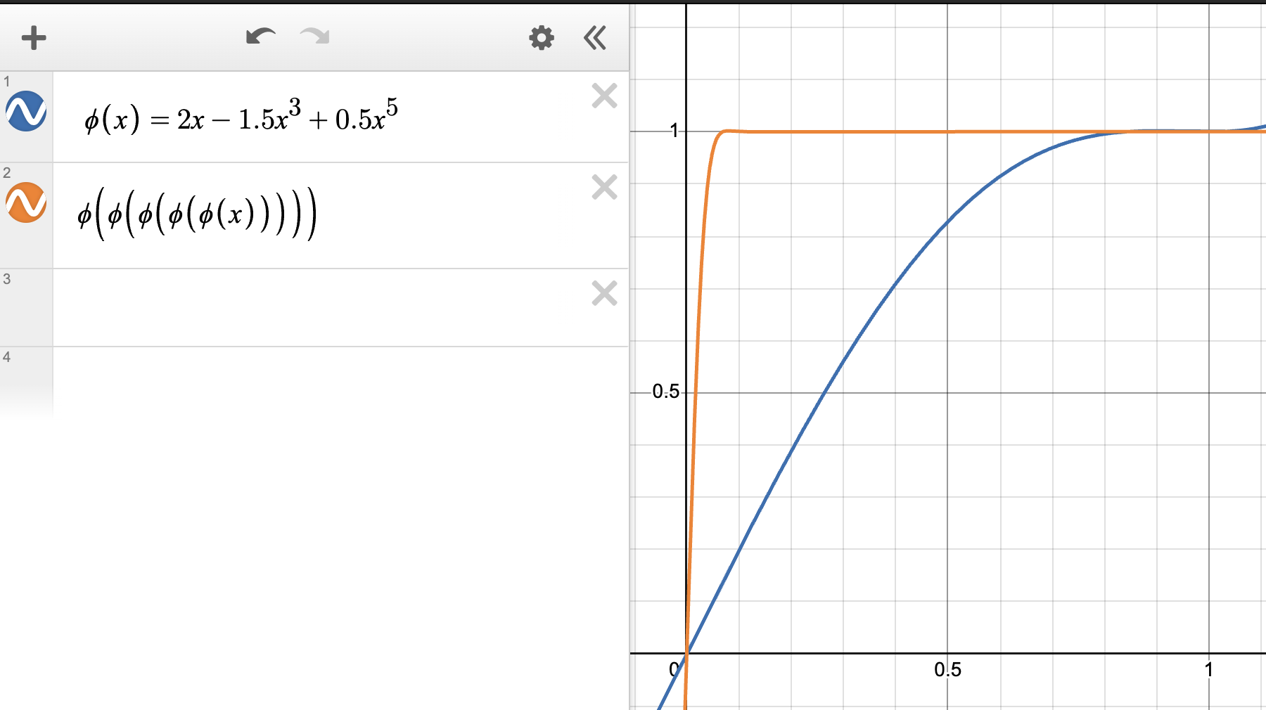 Baseline quintic polynomial \(\phi(s) = as + bs^3 + cs^5\) applied iteratively: singular values converge toward 1 but require several iterations with the default coefficients.
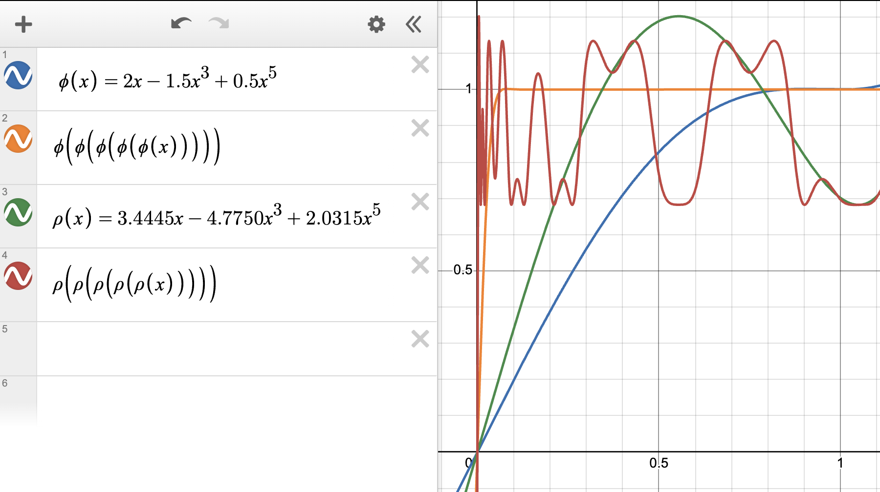 Optimized Newton-Schulz coefficients exhibiting steeper growth near \(s = 0\), achieving faster convergence to 1 in fewer iterations — the coefficients \((a, b, c) = (3.4445, -4.7750, 2.0315)\) used in practice.
A cubic polynomial \(\phi(s) = as + bs^3\) only has two degrees of freedom, limiting convergence speed. The quintic adds a fifth-degree term, giving faster convergence toward sign\((s) = 1\) for \(s > 0\). The coefficients \((a, b, c)\) are optimized numerically to minimize the number of iterations required for convergence to within 0.3 over \([0, 1]\).
FLOP overhead. Each Newton-Schulz step requires computing \(\mathbf{X}_k\mathbf{X}_k^\top \in \mathbb{R}^{m \times m}\) and then two subsequent multiplications. The total FLOP overhead relative to the forward/backward pass is:
\[\text{overhead} = \frac{T \cdot m}{B}\]
where \(T = 5\) is the number of NS iterations, \(m\) is the model dimension, and \(B\) is the batch size in tokens. For typical settings (NanoGPT: \(\sim 0.7\%\); Llama 405B: \(\sim 0.5\%\)).
2.3 Scaled Muon for Large Models
⚠️ The basic Muon algorithm produces updates of inconsistent root-mean-square (RMS) magnitude depending on the shape of the parameter matrix. The Kimi team identifies this as the primary obstacle to scalability.
Lemma (Liu et al., 2025). For a full-rank weight matrix \(\mathbf{W} \in \mathbb{R}^{A \times B}\), the theoretical update RMS under the basic Muon rule is:
\[\operatorname{RMS}(\mathbf{O}) = \frac{1}{\sqrt{\max(A, B)}}\]
Proof sketch. \(\mathbf{O} = \mathbf{U}\mathbf{V}^\top\) has \(\min(A, B)\) singular values all equal to 1. The Frobenius norm is \(\|\mathbf{O}\|_F = \sqrt{\min(A, B)}\). The RMS is \(\|\mathbf{O}\|_F / \sqrt{AB} = \sqrt{\min(A,B)/AB} = 1/\sqrt{\max(A,B)}\).
This means Muon naturally applies smaller-RMS updates to larger matrices — a shape-dependent bias. The fix is a rescaling:
The scaled Muon update (MuonW):
\[\mathbf{W}_t = \mathbf{W}_{t-1} - \eta_t \left(0.2 \cdot \mathbf{O}_t \cdot \sqrt{\max(A, B)} + \lambda \mathbf{W}_{t-1}\right)\]
The factor \(0.2\sqrt{\max(A,B)}\) restores a target RMS of \(0.2\), matching AdamW’s typical effective update scale. The \(\lambda \mathbf{W}_{t-1}\) term is standard decoupled weight decay.
Muon is designed for 2D weight matrices in linear layers. Embedding tables, classifier heads, 1D bias vectors, and layer norm parameters should use AdamW instead. The QKV projection matrices should have their Q, K, V portions treated as separate matrices (not concatenated) if their feature spaces are semantically distinct.
3. Derivation from First Principles
📐 The following derivation, due to Jeremy Bernstein, shows that the Muon update is not heuristic — it is the exact solution to a principled constrained optimization problem.
3.1 Metrizing the Linear Layer
Definition (RMS norm). For a vector \(\mathbf{v} \in \mathbb{R}^d\), the root-mean-square norm is: \[\|\mathbf{v}\|_{\text{RMS}} := \sqrt{\frac{1}{d} \sum_{i=1}^d v_i^2} = \frac{\|\mathbf{v}\|_2}{\sqrt{d}}\]
The RMS norm measures “average entry size” rather than total magnitude. For activations in a well-initialized network, \(\|\mathbf{x}\|_{\text{RMS}} \approx 1\) throughout training.
Definition (RMS-to-RMS operator norm). For a linear map \(\mathbf{W} : \mathbb{R}^{d_{\text{in}}} \to \mathbb{R}^{d_{\text{out}}}\), define: \[\|\mathbf{W}\|_{\text{RMS}\to\text{RMS}} := \max_{\mathbf{x} \neq 0} \frac{\|\mathbf{W}\mathbf{x}\|_{\text{RMS}}}{\|\mathbf{x}\|_{\text{RMS}}} = \sqrt{\frac{d_{\text{in}}}{d_{\text{out}}}} \cdot \|\mathbf{W}\|_{\text{op}}\]
where \(\|\mathbf{W}\|_{\text{op}} = \sigma_{\max}(\mathbf{W})\) is the spectral norm (largest singular value).
Derivation. Write \(\|\mathbf{W}\mathbf{x}\|_{\text{RMS}} = \|\mathbf{W}\mathbf{x}\|_2 / \sqrt{d_{\text{out}}}\) and \(\|\mathbf{x}\|_{\text{RMS}} = \|\mathbf{x}\|_2 / \sqrt{d_{\text{in}}}\). The ratio is \(({\sqrt{d_{\text{in}}}}/{\sqrt{d_{\text{out}}}}) \cdot (\|\mathbf{W}\mathbf{x}\|_2 / \|\mathbf{x}\|_2)\). Maximizing over \(\mathbf{x}\) gives \(\sqrt{d_{\text{in}}/d_{\text{out}}} \cdot \sigma_{\max}(\mathbf{W})\).
 The operator norm (spectral norm) measures the maximum factor by which a matrix can stretch an input vector — geometrically, the radius of the ellipsoid image of the unit sphere.
3.2 Steepest Descent Under the Operator Norm
The standard gradient descent update \(\mathbf{W} \leftarrow \mathbf{W} - \eta \nabla_\mathbf{W} \mathcal{L}\) is steepest descent under the Frobenius norm constraint \(\|\Delta\mathbf{W}\|_F \leq \eta\). Muon instead uses steepest descent under the RMS-to-RMS operator norm constraint.
Steepest descent means: given a step-size budget \(\eta\), choose the update \(\Delta\mathbf{W}\) that decreases the loss as much as possible. Under a first-order (linearization) approximation, the loss change is: \[\mathcal{L}(\mathbf{W} + \Delta\mathbf{W}) \approx \mathcal{L}(\mathbf{W}) + \langle \nabla_\mathbf{W}\mathcal{L},\, \Delta\mathbf{W} \rangle_F\] where \(\langle \mathbf{A}, \mathbf{B} \rangle_F = \operatorname{tr}(\mathbf{A}^\top \mathbf{B})\) is the Frobenius inner product. The steepest descent problem is therefore: \[\Delta\mathbf{W}^* = \arg\min_{\|\Delta\mathbf{W}\|_F \leq \eta} \langle \nabla_\mathbf{W}\mathcal{L},\, \Delta\mathbf{W} \rangle_F\] By the Cauchy–Schwarz inequality for the Frobenius inner product, \(\langle \mathbf{G}, \Delta\mathbf{W} \rangle_F \geq -\|\mathbf{G}\|_F \|\Delta\mathbf{W}\|_F\), with equality exactly when \(\Delta\mathbf{W} = -c\,\mathbf{G}\) for some \(c > 0\). The constraint \(\|\Delta\mathbf{W}\|_F \leq \eta\) then pins \(c = \eta / \|\mathbf{G}\|_F\), giving \(\Delta\mathbf{W}^* = -\eta\,\mathbf{G}/\|\mathbf{G}\|_F\). Up to the step-size normalisation (absorbed into \(\eta\)), this is exactly the gradient descent update \(-\eta\,\nabla_\mathbf{W}\mathcal{L}\).
The Frobenius norm treats every entry of \(\mathbf{W}\) symmetrically — it is the flat Euclidean metric on the space of matrices. Gradient descent is therefore the right steepest descent method if and only if Euclidean distance is the right measure of how much the weight matrix has changed. The key insight motivating Muon is that Euclidean distance in weight space is not a natural measure of change for a linear layer: what matters is how much the layer’s input–output behavior changes, which is measured by the operator norm, not the Frobenius norm.
 Choosing the right geometry for weight updates: Frobenius norm (SGD), element-wise \(\ell^\infty\) (Adam), or operator norm (Muon) each induce different steepest descent directions and distinct optimization theories.
Problem formulation. Given the linearized loss \(\langle \nabla_\mathbf{W}\mathcal{L}, \Delta\mathbf{W}\rangle\), find:
\[\Delta\mathbf{W}^* = \arg\min_{\Delta\mathbf{W}} \langle \nabla_\mathbf{W}\mathcal{L}, \Delta\mathbf{W}\rangle \quad \text{subject to} \quad \|\Delta\mathbf{W}\|_{\text{RMS}\to\text{RMS}} \leq \eta\]
Since \(\|\Delta\mathbf{W}\|_{\text{RMS}\to\text{RMS}} = \sqrt{d_{\text{in}}/d_{\text{out}}} \cdot \sigma_{\max}(\Delta\mathbf{W})\), this is equivalent to constraining the spectral norm \(\sigma_{\max}(\Delta\mathbf{W}) \leq \eta \sqrt{d_{\text{out}}/d_{\text{in}}}\).
3.3 The Dual Solution is UV^T
Proposition. Let \(\mathbf{G} = \nabla_\mathbf{W}\mathcal{L} \in \mathbb{R}^{d_{\text{out}} \times d_{\text{in}}}\) with SVD \(\mathbf{G} = \mathbf{U}\boldsymbol{\Sigma}\mathbf{V}^\top\). The solution to the constrained steepest descent problem is:
\[\Delta\mathbf{W}^* = -\eta \sqrt{\frac{d_{\text{out}}}{d_{\text{in}}}} \cdot \mathbf{U}\mathbf{V}^\top\]
Proof. The dual norm of \(\|\cdot\|_{\text{op}}\) (spectral norm) is the nuclear norm \(\|\cdot\|_* = \sum_i \sigma_i\). By the duality of norms, the steepest descent direction under spectral norm constraint is the maximizer of:
\[\langle \mathbf{G}, \Delta\mathbf{W}\rangle \quad \text{subject to} \quad \|\Delta\mathbf{W}\|_{\text{op}} \leq c\]
The nuclear norm/spectral norm duality gives: \(\langle \mathbf{G}, \Delta\mathbf{W}\rangle \leq \|\mathbf{G}\|_* \cdot \|\Delta\mathbf{W}\|_{\text{op}}\), with equality when \(\Delta\mathbf{W} \propto \mathbf{U}\mathbf{V}^\top\). To see this: \(\langle \mathbf{G}, \mathbf{U}\mathbf{V}^\top\rangle = \operatorname{tr}(\mathbf{V}\mathbf{U}^\top \mathbf{U}\boldsymbol{\Sigma}\mathbf{V}^\top) = \operatorname{tr}(\boldsymbol{\Sigma}) = \|\mathbf{G}\|_*\), which is maximal. The scaling \(\sqrt{d_{\text{out}}/d_{\text{in}}}\) comes from the RMS-to-RMS normalization factor. \(\square\)
Key conclusion: the Muon update direction \(\mathbf{U}\mathbf{V}^\top\) is the exact steepest descent direction under the RMS-to-RMS operator norm constraint on weight perturbations.
Suppose \(\mathbf{G} = \begin{pmatrix} 10 & 0 \\ 0 & 1 \end{pmatrix}\). Standard gradient descent takes a large step in the first singular direction and a tiny step in the second. Muon takes \(\mathbf{O} = \mathbf{I}\), an equal step in both directions. Under the spectral norm constraint, the second direction is “free” — we can take a full unit step there at no cost to the constraint budget.
3.4 Learning Rate Transfer Across Width
🔑 A critical practical consequence: steepest descent under the RMS-to-RMS operator norm automatically achieves maximal update parameterization (muP) learning rate transfer across model width.
Heuristic argument. In muP, the correct learning rate for a weight matrix scales as \(1/\text{fan\_in}\). The RMS-to-RMS operator norm includes a factor \(\sqrt{d_{\text{in}}/d_{\text{out}}}\), which under the steepest descent normalization produces a \(\sqrt{d_{\text{out}}/d_{\text{in}}}\) scaling in \(\Delta\mathbf{W}^*\). This matches the muP prescription: updates should be \(O(1/\sqrt{d_{\text{in}}})\) in RMS, independent of width, which is achieved by the polar factor \(\mathbf{U}\mathbf{V}^\top\) (whose RMS is \(\sim 1/\sqrt{\max(d_{\text{out}}, d_{\text{in}})}\) — the Lemma from §2.3).
 Empirical validation of learning rate transfer: dualized training (operator-norm steepest descent, equivalent to Muon) maintains consistent loss across model widths without retuning, while conventional training requires width-specific learning rates.
4. Connection to Shampoo and Second-Order Methods
🔗 The Shampoo optimizer maintains Kronecker-factored approximations of the gradient covariance and applies their inverse square-root as a preconditioner. Concretely, for \(\mathbf{G} \in \mathbb{R}^{m \times n}\), Shampoo computes:
 The Shampoo update rule: accumulate gradient outer products \(\mathbf{L}_t, \mathbf{R}_t\) and precondition with their inverse fourth roots. Muon recovers this update in the limiting case where all gradient history is discarded.
\[\mathbf{L}_t = \sum_{s \leq t} \mathbf{G}_s \mathbf{G}_s^\top \in \mathbb{R}^{m \times m}, \quad \mathbf{R}_t = \sum_{s \leq t} \mathbf{G}_s^\top \mathbf{G}_s \in \mathbb{R}^{n \times n}\]
and applies the update:
\[\Delta\mathbf{W} \propto -\mathbf{L}_t^{-1/4} \mathbf{G}_t \mathbf{R}_t^{-1/4}\]
Connection to Muon. Now suppose the gradient has no memory across steps: \(\mathbf{G}_s \approx \mathbf{G}_t\) for all \(s\). Then:
\[\mathbf{L}_t \approx T \cdot \mathbf{G}_t\mathbf{G}_t^\top = T \cdot \mathbf{U}\boldsymbol{\Sigma}^2\mathbf{U}^\top\]
\[\mathbf{L}_t^{-1/4} \approx T^{-1/4} \cdot \mathbf{U}\boldsymbol{\Sigma}^{-1/2}\mathbf{U}^\top\]
Similarly, \(\mathbf{R}_t^{-1/4} \approx T^{-1/4} \cdot \mathbf{V}\boldsymbol{\Sigma}^{-1/2}\mathbf{V}^\top\). Substituting:
\[\mathbf{L}_t^{-1/4}\mathbf{G}_t\mathbf{R}_t^{-1/4} \approx T^{-1/2} \cdot \mathbf{U}\boldsymbol{\Sigma}^{-1/2}\mathbf{U}^\top \cdot \mathbf{U}\boldsymbol{\Sigma}\mathbf{V}^\top \cdot \mathbf{V}\boldsymbol{\Sigma}^{-1/2}\mathbf{V}^\top = T^{-1/2} \cdot \mathbf{U}\mathbf{V}^\top\]
Muon is a limiting case of Shampoo where gradient memory is reset each step. This connection shows that Muon is implicitly doing approximate second-order preconditioning.
Shampoo requires maintaining and inverting the \(m \times m\) and \(n \times n\) covariance matrices, costing \(O(m^3 + n^3)\) per step (or using approximations). Muon’s Newton-Schulz iteration acts directly on \(\mathbf{G} \in \mathbb{R}^{m \times n}\) using matrix multiplications, with no explicit covariance accumulation. The computational savings are substantial for large matrices.
Muon discards all history of the gradient direction and uses only the current momentum buffer. Shampoo accumulates gradient outer products over many steps. Whether a variant of Muon that accumulates some spectral memory across steps could improve further is an open research direction.
5. The Geometric Interpretation: Hyperball Optimization
🔵 The hyperball perspective, developed by Wen (2025), frames Muon as optimizing on a constrained manifold to achieve designed rather than accidental update-to-weight ratios.
The instability of standard optimizers. In AdamW and SGD, the ratio \(\|\mathbf{u}_t\|_F / \|\mathbf{W}_t\|_F\) (where \(\mathbf{u}_t\) is the raw update before scaling by \(\eta\)) evolves unpredictably across layers, widths, and depths. The effective step size along each eigen-direction depends on accumulated gradient statistics in ways that are hard to control.
The hyperball normalization scheme. Define normalization to a sphere of radius \(R\) as:
\[\operatorname{Normalize}_R(\mathbf{X}) := R \cdot \frac{\mathbf{X}}{\|\mathbf{X}\|_F}\]
The hyperball update rule is:
\[\mathbf{W}_{t+1} = \operatorname{Normalize}_R\!\left(\mathbf{W}_t - \eta \cdot \operatorname{Normalize}_R(\mathbf{u}_t)\right)\]
where \(R = \|\mathbf{W}_0\|_F\) is fixed at initialization. This ensures:
- Weight norms are pinned: \(\|\mathbf{W}_t\|_F = R\) for all \(t\).
- Update norms are pinned: \(\|\text{applied update}\|_F = \eta\) for all \(t\).
- The ratio \(\eta / R\) is the designed step size, predictable and transferable.
Connection to Muon. The “normalize the update” step \(\operatorname{Normalize}_R(\mathbf{u}_t)\) applied to a matrix generalizes naturally to matching the singular vectors rather than just the Frobenius norm. Specifically, if one further constrains the update to lie on the Stiefel manifold (the set of semi-orthogonal matrices), the minimum-distortion lift from a vector update to a matrix update is exactly \(\mathbf{U}\mathbf{V}^\top\).
Practical benefit. By pinning the update-to-weight ratio to a designed constant, hyperball optimization enables hyperparameter transfer across model width and depth without muP reparameterization.
 Empirical performance of the Hyperball optimizer relative to AdamW and MuonW: by enforcing a hard norm constraint on both weights and updates, Hyperball achieves faster convergence and improved sample efficiency.
Hyperball normalization also normalizes the weights themselves (projecting \(\mathbf{W}_t\) back onto a sphere at each step). Standard Muon does not do this — it only orthogonalizes the update, not the weights. The weight decay term in MuonW provides a soft analogue: it prevents weight norms from growing unboundedly, but does not enforce a hard norm constraint.
6. The Explore-Exploit Perspective
🗺️ An alternative lens, developed by Paperplanet (2025), interprets Muon’s update as balancing exploration of gradient directions against exploitation of the steepest-descent path.
The exploit-only baseline. Standard gradient descent (and Adam) follow the gradient direction, concentrating the update budget on singular directions with large singular values. If \(\mathbf{G} = \mathbf{U}\boldsymbol{\Sigma}\mathbf{V}^\top\), then:
\[\text{Adam update} \approx -\mathbf{U}\operatorname{sign}(\boldsymbol{\Sigma})\mathbf{V}^\top \quad \text{(element-wise sign adaptation)}\]
In practice, Adam’s sign operation on individual entries does not align with the SVD structure, but the effect is qualitatively similar: it amplifies directions according to gradient magnitude.
Muon’s exploration. By normalizing all singular values to 1:
\[\mathbf{O}_t = \sum_{i=1}^r \mathbf{u}_i \mathbf{v}_i^\top\]
Muon assigns equal priority to every singular direction, regardless of whether the corresponding singular value is large or small. This forces the optimizer to explore directions where the current gradient signal is weak — which may correspond to important but currently dormant features.
Why exploitation is still present. The gradient \(\mathbf{G}\) determines the singular vectors \(\mathbf{u}_i, \mathbf{v}_i\). These encode the direction of the gradient in the input/output feature spaces. Muon exploits this directional information fully while ignoring the magnitude information. Subsequent gradient computations (at the next step) naturally correct any overshooting from over-weighted minor directions.
Empirical signature. The Kimi team observes that “SVD entropy of Muon is higher than that of AdamW” across training checkpoints — confirming that Muon uses more of the available singular directions, consistent with the exploration interpretation.
 The end-to-end computational process of Muon: the gradient is smoothed via momentum, normalized to unit Frobenius norm, passed through Newton-Schulz iteration to recover the polar factor \(\mathbf{U}\mathbf{V}^\top\), and scaled before application.
In mixture-of-experts architectures, the router weight matrices have strongly peaked singular value spectra: a few directions dominate expert routing. Adam reinforces these dominant directions, while Muon forces exploration of alternative routing patterns. This may explain why Moonlight (trained with Muon) shows particularly large gains on reasoning tasks like MATH, which may require activating diverse expert combinations.
7. Su Jianlin’s Spectral Norm Perspective
📐 Jianlin Su’s analysis (kexue.fm) provides an independent angle: characterizing what norm Muon is steepest descent under and contrasting it with AdamW.
AdamW’s implicit norm. AdamW with element-wise second-moment normalization is approximately steepest descent under the max-of-max norm — which normalizes each parameter element individually. This is a very weak norm that treats all matrix entries symmetrically.
Muon’s implicit norm. As derived in §3, Muon is steepest descent under the spectral norm (or equivalently, the RMS-to-RMS operator norm). The spectral norm is the natural norm for linear operators acting on Euclidean space, since it measures the maximum amplification factor applied to inputs.
Why the spectral norm is the right choice. Weight matrices in neural networks function as linear operators: they map activation vectors from one representation space to another. The spectral norm measures the worst-case distortion of this mapping. An update constrained to be small in spectral norm guarantees that the network’s input-output behavior changes in a controlled way, regardless of the direction.
The Frobenius norm (used by SGD) treats all singular directions equally and may allow large changes in the network’s behavior (by making a large change in a dominant singular direction). The spectral norm provides a tighter coupling between weight change and behavioral change.
The dual norm of the spectral norm is the nuclear norm \(\|\mathbf{G}\|_* = \sum_i \sigma_i(\mathbf{G})\). The steepest descent direction under a norm constraint \(\|\Delta\mathbf{W}\|_{\text{op}} \leq \eta\) is the subdifferential of the dual norm at \(\mathbf{G}\), which is exactly \(\mathbf{U}\mathbf{V}^\top\) (a subgradient of the nuclear norm). This is a standard result in convex analysis.
Frobenius vs. spectral norm comparison:
| Constraint | Dual norm | Steepest descent direction | Method |
|---|---|---|---|
| \(\|\Delta\mathbf{W}\|_F \leq \eta\) | Frobenius | \(-\mathbf{G}\) | SGD |
| \(\|\Delta\mathbf{W}\|_{\text{op}} \leq \eta\) | Nuclear | \(-\mathbf{U}\mathbf{V}^\top\) | Muon |
| Element-wise \(\ell^\infty\) | \(\ell^1\) | \(-\operatorname{sign}(\mathbf{G})\) | Adam (approx.) |
8. Why Orthogonalization Helps in Practice
💡 Several independent empirical and theoretical observations explain why replacing the gradient with its polar factor improves training.
High condition numbers of transformer gradients. Gradient matrices in transformers tend to have high condition numbers — the ratio of largest to smallest singular value is very large. This means gradient descent allocates almost all of its update budget to a few dominant directions, making extremely slow progress in the remaining directions.
Orthogonalization effectively sets the condition number of the update to 1. Every singular direction receives equal treatment. This counters the “gradient concentration” pathology.
Rare but important directions. The minor singular directions of the gradient (those with small \(\sigma_i\)) correspond to weight perturbations that the loss is currently insensitive to — but they may be highly relevant for long-range optimization. By amplifying these directions equally with the dominant ones, Muon ensures they are not neglected.
Watermark erasure as a diagnostic. Bernstein’s analysis notes that models trained with Muon show faster erasure of training data watermarks — meaning the weights move substantially from initialization. This indicates that Muon is genuinely exploring the weight space rather than staying near the NTK (neural tangent kernel) regime.
SVD entropy. The Kimi team measures that Muon-trained models consistently have higher SVD entropy (defined as \(-\sum_i \bar\sigma_i \log \bar\sigma_i\) where \(\bar\sigma_i = \sigma_i / \sum_j \sigma_j\) are normalized singular values) in their weight matrices. Higher entropy means more evenly distributed singular value spectra — the model is using more of its representational capacity.
 Singular value distributions of transformer attention weight matrices across training: weights remain close to full rank rather than collapsing to a low-rank structure, supporting the claim that orthogonalization encourages uniform use of representational capacity.
Muon orthogonalizes the update, not the weights. After one Muon step, \(\mathbf{W}_t - \eta \mathbf{U}\mathbf{V}^\top\) is not in general a well-conditioned matrix. What Muon controls is the update direction — ensuring that the step taken in weight space is balanced across singular directions.
9. Distributed Implementation
🖥️ A significant engineering contribution of Liu et al. (2025) is a memory-optimal, communication-efficient distributed implementation for Megatron-LM.
The challenge is that Newton-Schulz requires the full gradient matrix \(\mathbf{M}_t \in \mathbb{R}^{m \times n}\) for orthogonalization, but in distributed training each device holds only a shard of each parameter matrix. Naive approaches would either (a) replicate the full gradient on all devices (memory-prohibitive) or (b) apply NS to each shard independently (mathematically incorrect — the polar factor of a submatrix is not a submatrix of the polar factor).
Algorithm (Distributed Muon):
flowchart TD
    A["Gradient shards G_i
on each DP rank"] --> B["AllGather across DP group
assembles full G"]
    B --> C["Newton-Schulz on full G
produces full O = UV^T"]
    C --> D["Each rank discards
non-local rows/cols of O"]
    D --> E["Apply local shard
of O to local W shard"]
- DP Gather: Assemble partitioned gradient shards into the full gradient \(\mathbf{G}\).
- Full NS: Compute \(\mathbf{O} = \operatorname{NS}(\mathbf{G})\) on each device (redundant but necessary for correctness).
- Selective discard: Each device retains only the rows/columns of \(\mathbf{O}\) corresponding to its local parameter shard.
Communication cost. The only extra communication is the AllGather of gradients within DP groups. The additional overhead is \([1, 1.25]\times\) that of AdamW, with practical overhead near the lower bound \(1\times\) when multiple DP groups are used.
AdamW requires storing two optimizer states (first and second moment) per parameter. Muon requires storing only the momentum buffer (one state per parameter). The orthogonalized update \(\mathbf{O}\) is computed on-the-fly and not stored. Muon therefore uses approximately half the optimizer state memory of AdamW.
10. Practical Considerations and Hyperparameters
🔧 The following table summarizes recommended hyperparameters for MuonW (the scaled, weight-decayed Muon variant):
| Hyperparameter | Recommended Value | Notes |
|---|---|---|
| Momentum \(\mu\) | 0.95 | Higher than typical 0.9 for SGD |
| NS iterations \(N\) | 5 | \(N = 10\) gives negligible improvement |
| NS coefficients \((a,b,c)\) | \((3.4445, -4.7750, 2.0315)\) | Optimized quintic |
| Update RMS scale | 0.2 | Matches AdamW’s typical effective scale |
| Weight decay \(\lambda\) | 0.1 | Critical for stability at scale |
| Learning rate | Reuse AdamW’s | Transfers directly with the RMS scaling |
Which parameters to apply Muon to:
flowchart TD
    P["Parameter tensor"] --> D{"2D weight matrix?"}
    D -->|"yes"| E{"Embedding or
classifier head?"}
    E -->|"no"| F["Apply MuonW"]
    E -->|"yes"| G["Apply AdamW"]
    D -->|"no"| H["Apply AdamW
(biases, norms, 1D params)"]
QKV handling. For attention QKV projections stored as a single concatenated matrix \([\mathbf{W}_Q; \mathbf{W}_K; \mathbf{W}_V]\), apply NS to each of the three sub-matrices independently. Treating the full concatenation as a single matrix is incorrect because Q, K, V operate in different semantic spaces.
SFT compatibility. Models pretrained with Muon should also be fine-tuned with Muon. The Kimi team observes that switching from Muon pretraining to AdamW fine-tuning yields no significant advantage over AdamW-pretrained models. The optimizer mismatch degrades the Muon pretraining benefits.
Always normalize \(\mathbf{M}_t\) to unit Frobenius norm before running the NS iteration. Without normalization, singular values outside \([0, 1]\) cause the polynomial to diverge. The normalization factor is discarded after NS (the output \(\mathbf{O}\) has Frobenius norm \(\approx \sqrt{\min(m,n)}\), which is then corrected by the \(0.2\sqrt{\max(m,n)}\) scaling).
11. Experimental Results
📊 The Kimi team validates Muon on two axes: scaling law experiments (controlled FLOP comparisons) and the Moonlight production model.
Scaling law comparison. Under compute-optimal training (following Chinchilla scaling), Muon achieves:
\[\mathcal{L}_{\text{Muon}}(C) = 2.506 \times C^{-0.052}\] \[\mathcal{L}_{\text{AdamW}}(C) = 2.608 \times C^{-0.054}\]
At any fixed compute budget \(C\), Muon requires approximately 52% of AdamW’s FLOPs to reach the same loss. This is the headline 2x efficiency result.
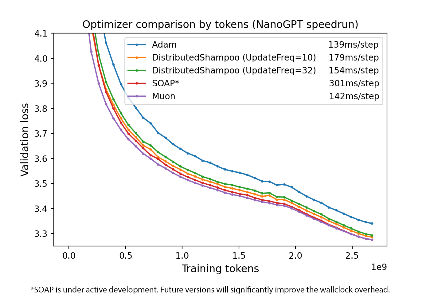 Sample efficiency comparison across optimizers on the NanoGPT speedrun benchmark: Muon reaches target validation loss with significantly fewer training tokens than AdamW, SGD, and other baselines.
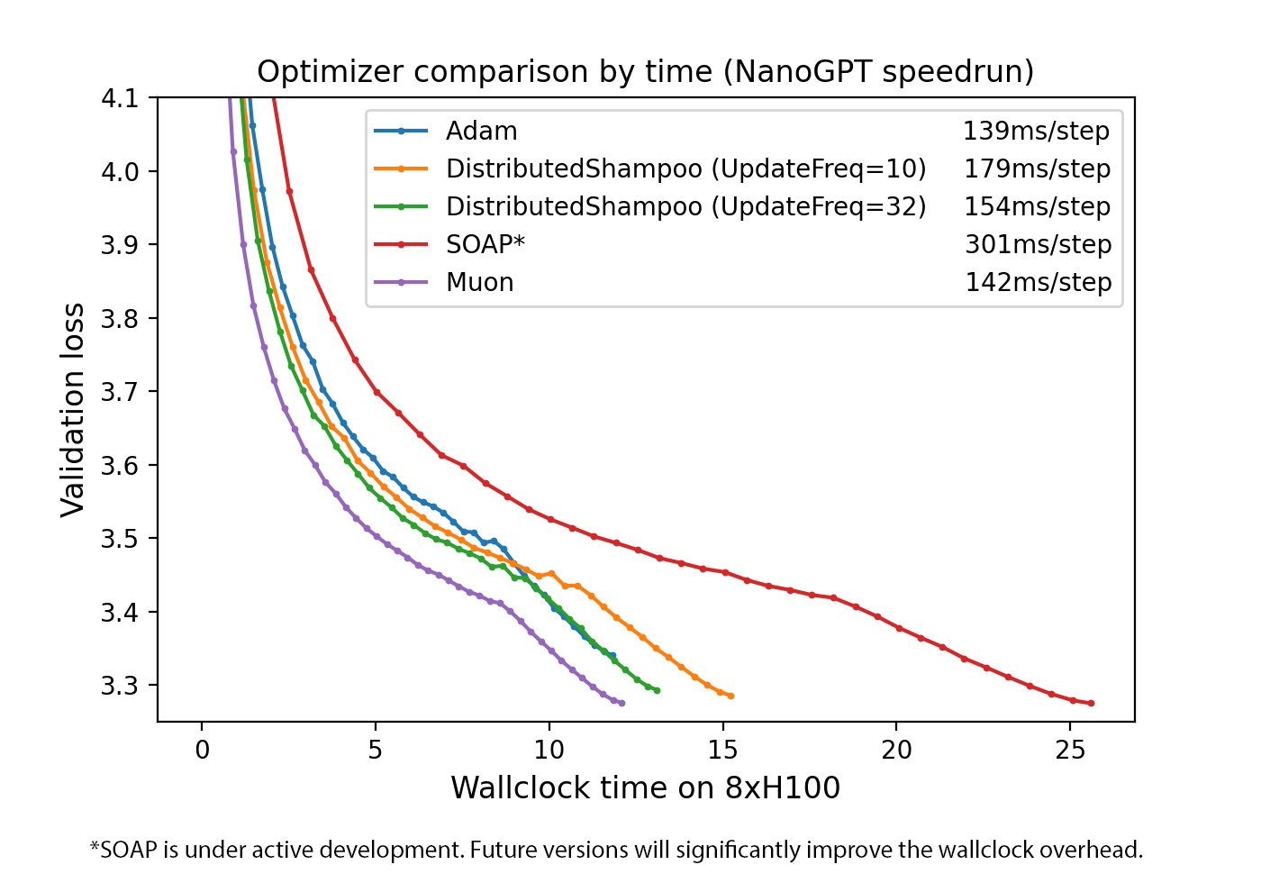 Wallclock training time comparison: despite the overhead of Newton-Schulz iterations (~0.7% extra FLOPs at NanoGPT scale), Muon reaches target loss faster in wall time due to its superior per-token progress.
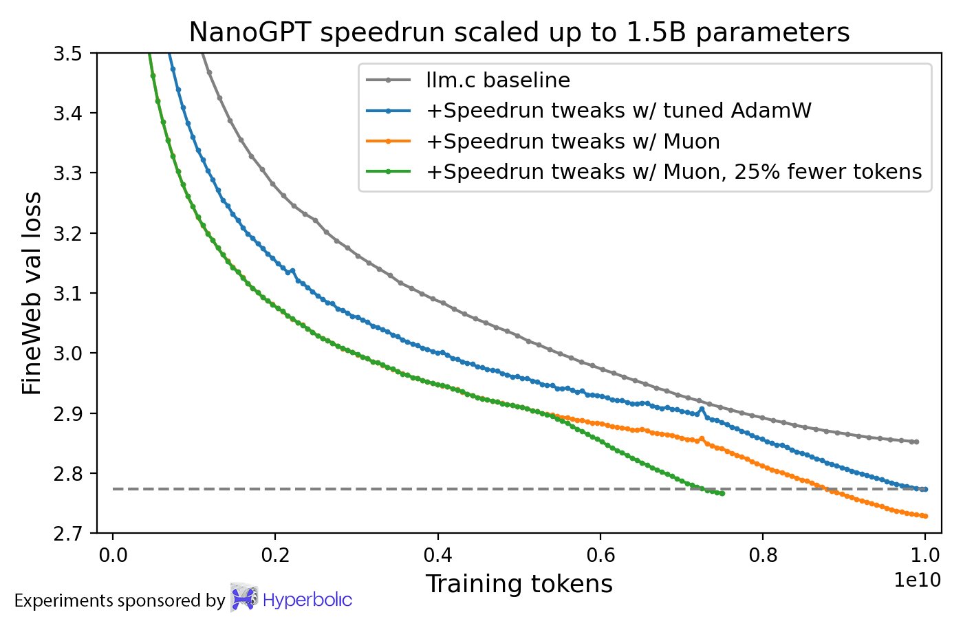 Scaling validation at 1.5B parameters: Muon maintains its loss advantage over AdamW at larger scale, establishing that the efficiency gain is not limited to small models.
Moonlight results (3B active / 16B total MoE, 5.7T tokens):
| Benchmark | DeepSeek-V2-Lite (AdamW) | Moonlight (Muon) |
|---|---|---|
| MMLU | 58.3 | 70.0 |
| MATH | 17.1 | 45.3 |
| HumanEval | 29.9 | 48.1 |
The comparison is same architecture, same number of training tokens.
Spectral analysis. Muon-trained models exhibit higher SVD entropy in weight matrices throughout training, with the effect most pronounced in MoE router weights. This is consistent with the explore-exploit analysis: Muon encourages more diverse routing patterns, which may underlie the large MATH and reasoning gains.
The 2x compute efficiency is measured under compute-optimal training, where both model size and token count are simultaneously optimized for a given FLOP budget. At fixed model size with increasing tokens (beyond the compute-optimal point), the advantage may differ. The paper does not report this regime.
12. The Modular Norm: Metrizing the Full Network
📐 The single-layer analysis of §3 shows that Muon is steepest descent under the RMS-to-RMS operator norm on one weight matrix. But a neural network has many weight matrices, and one still needs to decide how to aggregate layer-wise norms into a norm on the full parameter vector. The modular norm of Large et al. (2024) provides the principled answer.
12.1 From Layer Norms to Network Norms
Given layer-wise norms \(\|\cdot\|_{W_k}\) and scaling constants \(s_1, \ldots, s_L > 0\), the modular norm on the full weight space \(\mathcal{W} = \mathcal{W}_1 \times \cdots \times \mathcal{W}_L\) is:
\[\|(w_1, \ldots, w_L)\|_{\mathcal{W}} := \max_{k}\bigl(s_k \|w_k\|_{\mathcal{W}_k}\bigr)\]
This is an \(\ell^\infty\) combination of scaled layer norms — not an \(\ell^2\) or \(\ell^1\) combination. The choice of \(\ell^\infty\) is not aesthetic: it is forced by the requirement that the associated Lipschitz (sharpness) constant be invariant to depth. An \(\ell^2\) combination would produce a sharpness constant that grows with \(\sqrt{L}\), making learning rate transfer across depth impossible.
The recursive construction. The modular norm is built up from modules — composable objects that carry four attributes: forward, mass, sensitivity, and norm. Two binary operations suffice to build any architecture:
- Composition \(M_2 \circ M_1\): the composite norm is \(\max\!\bigl(M_2.\mathrm{sensitivity} \cdot \tfrac{M.\mathrm{mass}}{M_1.\mathrm{mass}} \|w_1\|_1,\, \tfrac{M.\mathrm{mass}}{M_2.\mathrm{mass}} \|w_2\|_2\bigr)\).
- Concatenation \((M_1, M_2)\): the norm is \(\max\!\bigl(\tfrac{M.\mathrm{mass}}{M_1.\mathrm{mass}} \|w_1\|_1,\, \tfrac{M.\mathrm{mass}}{M_2.\mathrm{mass}} \|w_2\|_2\bigr)\) (sensitivity does not appear because neither module feeds through the other).
The key invariant maintained throughout is well-normedness: a module is well-normed if \(\|\nabla_w M(w,x) \cdot \Delta w\|_Y \leq \|\Delta w\|_M\) (Lipschitz-1 in weight space) and \(\|\nabla_x M(w,x) \cdot \Delta x\|_Y \leq M.\mathrm{sensitivity} \cdot \|\Delta x\|_X\) (Lipschitz-sensitivity in input space). Both composition and concatenation preserve well-normedness.
Mass allocation. The mass parameter of each module controls the proportion of feature learning that module contributes to any compound module. If \(M_k.\mathrm{mass} / M.\mathrm{mass}\) is the fraction of total mass assigned to layer \(k\), then the contribution of that layer to the linearized output change is bounded by that same fraction times \(\|{}\Delta w\|_{\mathcal{W}}\). For residual networks, the empirically best choice keeps the total mass of hidden layers \(m\) fixed as depth scales (\(M_{\text{block}}.\mathrm{mass} = m/L\)), so that each block learns at rate \(O(1/L)\) and the total hidden-layer learning remains \(O(1)\).
Proposition (Large et al., 2024). For any neural network built from well-normed atomic modules — including linear layers (using the RMS-to-RMS operator norm), embedding layers (using the \(\ell^1 \to \ell^2\) max-column norm), and standard nonlinearities — the gradient of the network is Lipschitz-continuous in the modular norm, with a sharpness constant that is independent of depth for residual networks with the canonical mass allocation. This is the rigorous foundation for depth-transferable learning rates.
12.2 The Anthology: Optimizers as Steepest Descent
Bernstein & Newhouse (2024) unify Adam, Shampoo, and Muon by showing that each (with exponential moving averages disabled) is steepest descent under a particular norm:
| Optimizer | Norm | Update direction |
|---|---|---|
| Adam (no EMA) | Max-of-max norm: \(\max_l \|W_l\|_{\ell^1 \to \ell^\infty}\) | \(-\operatorname{sign}(G_l)\) layer-wise |
| Shampoo / Muon (no accum.) | Max spectral norm: \(\max_l \|W_l\|_{\ell^2 \to \ell^2}\) | \(-U_l V_l^\top\) layer-wise |
| SGD | Frobenius (Schatten-2) norm | \(-G_l / \|G_l\|_F\) |
The max over layers is the \(\ell^\infty\) aggregation of the modular norm — both Adam and Shampoo/Muon implicitly use a modular norm, but with different choices of per-layer norm (\(\ell^1 \to \ell^\infty\) vs. \(\ell^2 \to \ell^2\)).
The steepest descent problem for the modular norm \(\max_l s_l \|\Delta W_l\|_l\) is:
\[\Delta W_l^* = -\frac{\eta}{s_l} \cdot \underset{\|T_l\|_l \leq 1}{\operatorname{arg\,max}}\langle G_l, T_l \rangle \qquad \text{with global step size } \eta = \frac{1}{\lambda}\sum_k s_k \|G_k\|_k^*\]
Each layer is updated in the direction of the steepest descent under its own norm, with a global learning rate shared across layers. This is precisely the recipe of both Muon (spectral norm per layer) and normed Adam (infinity norm per layer).
Once exponential moving averages are restored, Adam and Shampoo no longer exactly solve a steepest descent problem — the accumulated statistics introduce a bias toward historically large gradient directions. The norm interpretation is exact only in the no-EMA limit. Nevertheless, the anthology argues that EMA plays the role of “smoothing” rather than fundamentally changing the algorithm, and the norm perspective still guides intuition.
The modular norm assigns each layer its natural norm based on the role it plays. A linear layer \(W \in \mathbb{R}^{d_\text{out} \times d_\text{in}}\) maps RMS-normalized activations to RMS-normalized pre-activations, so the RMS-to-RMS operator norm (= rescaled spectral norm) is the tightest measure of behavioral change. Steepest descent under this norm gives \(\Delta W \propto UV^\top\) — precisely Muon.
12.3 Normed Optimization in Practice
The Modula Python package (available via pip install modula) implements the modular norm for arbitrary PyTorch architectures. The training loop becomes:
delta_w = base_optim.step(net.parameters())   # run Adam or SGD
net.normalize(delta_w)                         # normalize in modular norm
net.parameters() -= eta(step) * delta_w        # apply with LR schedule
The normalization wrapper renders the optimal learning rate invariant to width and depth, with no muP-style correction factors. Empirically:
- Learning rate sweeps collapse to the same optimum across width \(2^5\)–\(2^8\) and depth \(2\)–\(10\) blocks.
- Normed SGD trains GPT on par with AdamW, at half the memory (no second moment needed).
- Mass hyperparameter: best performance at \(m \approx 0.5\)–\(1\) for residual MLP on CIFAR-10; transferable from small to large scale.
Computing the normalization requires evaluating each layer’s norm (e.g., spectral norm for linear layers). Spectral norm computation costs \(O(\min(d_\text{in}, d_\text{out}))\) via a power iteration or \(O(d_\text{in} d_\text{out} \min(d_\text{in}, d_\text{out}))\) via SVD. In practice, one or two steps of power iteration suffice and the overhead is small, but it is nonzero — unlike Muon’s Newton-Schulz approach, which handles orthogonalization and normalization simultaneously.
12.4 Why Embedding Layers Need a Different Norm
🔑 The Muon paper prescribes AdamW for embedding tables but Muon for linear layers — a distinction that the modular norm makes theoretically precise.
An embedding layer maps a one-hot token index \(e_i \in \{0,1\}^V\) (with \(\|e_i\|_1 = 1\)) to a dense embedding \(We_i \in \mathbb{R}^d\). The natural input norm is \(\ell^1\) (not \(\ell^2\), since activations are one-hot). The induced operator norm is therefore the \(\ell^1 \to \ell^2\) norm:
\[\|W\|_{\ell^1 \to \ell^2} = \max_j \|W_{:,j}\|_2 \qquad \text{(max column norm)}\]
The steepest descent direction under the max-column norm is not \(UV^\top\) — it is a per-column normalization that corresponds more closely to Adam (sign-like) behavior on embedding rows. This is why AdamW, which approximates per-element normalization, is more suitable for embeddings than Muon.
In summary: the modular norm assigns \(\|\cdot\|_{\ell^2 \to \ell^2}\) (spectral) to linear layers and \(\|\cdot\|_{\ell^1 \to \ell^2}\) (max-column) to embedding layers. Muon implements spectral steepest descent; Adam implements a max-norm approximation. The modular norm is the framework that explains why you use one and not the other.
The family of Schatten norms \(S_p\) interpolates between the spectral norm (\(S_\infty = \sigma_\max\)), the Frobenius norm (\(S_2 = \|\sigma\|_2\)), and the nuclear norm (\(S_1 = \sum_i \sigma_i\)). The Bernstein anthology notes that steepest descent under \(S_\infty\) (spectral) gives \(UV^\top\) (Muon / Shampoo), while steepest descent under \(S_2\) (Frobenius) gives \(G/\|G\|_F\) (standard gradient descent). The modular norm chooses \(S_\infty\) per layer (the max Schatten norm over layers) as the architecture-aware norm for multi-layer networks.
13. External Validation and Scaling Limits
⚠️ The Kimi team’s experimental results (§11) show Muon outperforming AdamW by 2× in compute efficiency. This figure requires scrutiny. A systematic independent benchmark by Wen et al. (2025) — covering 11 optimizers, 4 model scales, and 4 Chinchilla regimes with rigorous per-optimizer hyperparameter tuning — reveals that the true picture is both more nuanced and more honest.
13.1 Correcting the Speedup Claim
The 2× figure in the Kimi paper, and similar claims in concurrent works, share a common methodological flaw: the AdamW baseline is undertuned. The standard GPT-3 recipe uses a peak learning rate of 6e-4. Wen et al. show that tuning only the learning rate for AdamW — moving from 6e-4 to 8e-3 — already produces a ~2× speedup on a 130M model. In other words, the “2×” gain attributed to Muon is largely the gain of comparing against a misconfigured baseline.
Against a properly tuned AdamW (via exhaustive coordinate descent on all hyperparameters), Muon’s actual measured speedup is:
| Model size | Chinchilla ratio | Muon speedup vs. AdamW |
|---|---|---|
| 130M | 1–4× | ~1.3–1.4× |
| 300M–520M | 1–4× | ~1.3× |
| 1.2B | 1–8× | ~1.1× |
| 7B (extrapolated) | 1× | ≲1.0× (projected) |
The speedup is real but modest, and inversely proportional to model scale.
The 2× speedup claim propagated across many optimizer papers (MARS, Cautious, FOCUS, SWAN, DION all report ≥2×) because they shared the same undertuned GPT-3 recipe baseline. Wen et al. show that the maximum achievable speedup over a well-tuned AdamW is approximately 1.4× at any scale, and that this figure shrinks with model size. Comparing against a properly tuned baseline is non-negotiable for honest optimizer evaluation.
A secondary methodological issue: optimizer rankings can reverse during learning rate decay. Curves that show a large gap at intermediate checkpoints may flip before the end of training. This means early-stopping comparisons — common in the literature — are unreliable.
13.2 The Matrix-vs-Scalar Divide
Despite the corrected numbers, Wen et al. confirm the theoretically motivated prediction from §3 and §7: matrix-based optimizers are categorically better than scalar-based optimizers.
The benchmark groups optimizers into two families:
- Scalar-based (update each parameter independently using scalar operations): AdamW, NAdamW, MARS, Cautious, Lion, Adam-mini. After fair tuning, all scalar-based optimizers achieve similar performance to AdamW, with speedups of at most 1.2× over AdamW.
- Matrix-based (precondition gradients using matrix multiplication): Muon, Soap, Kron (PSGD), Scion. All matrix-based optimizers consistently outperform all scalar-based ones across every model scale and Chinchilla ratio tested.
This is a clean empirical validation of the theoretical narrative: the steepest descent under the spectral norm (§3.2–§3.3) is a genuinely better update rule for weight matrices than element-wise normalization (Adam) or plain gradient descent (SGD). The spectral norm is the right geometry for linear operators, and using it pays off across the board.
Within the matrix-based family, the methods share a common structure: each updates weight matrices by multiplying the gradient with a preconditioning matrix (rather than dividing element-wise by a scalar second moment). Muon uses Newton-Schulz to compute the polar factor; Soap uses Shampoo-style Kronecker preconditioning; Kron uses a different blocked Kronecker preconditioner. Despite different implementations, they converge to similar losses in the overtrained regime — suggesting the crucial ingredient is the matrix preconditioning itself, not the specific algorithm.
13.3 Scaling Limits: Model Size and Chinchilla Ratio
Two concrete failure modes are documented by Wen et al.
Failure mode 1: large models. Muon’s speedup over AdamW is inversely proportional to model size. At 1.2B parameters with 8× Chinchilla tokens, Muon achieves a speedup of only ~1.1× — statistically real but practically marginal. The fitted scaling law extrapolates to a slightly negative speedup for Muon vs. AdamW at 7B parameters in the 1× Chinchilla regime. This does not mean Muon is bad at scale — it means the matrix-based advantage that is clear at 100M parameters converges to roughly the same loss as AdamW at frontier model sizes. The current practical adoption at scale (e.g., Kimi K2 uses Muon-clip, a Muon variant) may reflect other benefits (optimizer state memory savings, distributional properties) rather than a speedup.
Failure mode 2: high data-to-model ratios. Muon is the best optimizer at 1–4× Chinchilla (the standard pretraining regime). But at 8–16× Chinchilla (heavily overtrained models, as used in Llama-3 style compute-optimal-then-continue setups), Muon is overtaken by Soap and Kron. The conjecture is that Soap and Kron, by maintaining accumulated gradient second-moment statistics (Kronecker preconditioners), become increasingly effective as the gradient signal is averaged over more data — while Muon, which discards gradient history at each step (see §4), loses relative to methods that exploit long-run gradient heterogeneity.
flowchart LR
    subgraph "Matrix-based optimizers"
    A["Muon
Best at 1–4× Chinchilla
Small-to-mid scale"]
    B["Soap / Kron
Best at ≥8× Chinchilla
High data ratio"]
    end
    C["Scalar-based
(AdamW, Lion, MARS)"]
    A -->|"overtrained regime"| B
    A -->|"always beats"| C
    B -->|"always beats"| C
If you are training in the compute-optimal (1× Chinchilla) regime or slightly beyond, Muon is the strongest matrix-based optimizer. If you are training a small model on a very large token budget (≥8× Chinchilla) — e.g., a 1B model on 200B+ tokens — Soap or Kron may be preferable. This regime dependence is not discussed in the original Muon papers.
13.4 Hyperparameter Sensitivity as Evidence for LR Transfer
One of Wen et al.’s key outputs is a table of scaling-sensitive hyperparameters for each optimizer — those that must be retuned as model size or data budget changes.
| Optimizer | Scaling-sensitive hyperparameters |
|---|---|
| AdamW | LR, warmup, weight decay, batch size |
| NAdamW | LR, warmup |
| Muon | LR only |
| Soap | LR, warmup, block size |
| Kron | LR |
Muon and Kron each have only one scaling-sensitive hyperparameter: the learning rate. This is direct empirical evidence for the LR transfer theory in §3.4. The modular norm derivation predicts that the Muon update direction (\(UV^\top\)) is intrinsically scale-normalized, so the only free parameter governing step size is \(\eta\) — and empirically, \(\eta\) must be retuned across scales but no other hyperparameter does. AdamW, by contrast, requires retuning weight decay and batch size in addition to LR, because its update direction is not intrinsically normalized.
For Muon: tune only the learning rate. The weight decay, momentum, and Newton-Schulz iterations are stable across scales. For the best results, use separate learning rates for embedding layers and matrix weights — the authors find this improves Muon’s performance non-trivially. The optimal LR for Muon at 520M scale is in the range 4e-3 to 8e-3, considerably higher than AdamW’s typical 6e-4.
References
| Reference Name | Brief Summary | Link to Reference |
|---|---|---|
| Muon is Scalable for LLM Training (Liu et al., 2025) | Primary paper; introduces MuonW with weight decay and per-parameter scaling, validates on Moonlight 3B/16B MoE, establishes 2x compute efficiency over AdamW | https://arxiv.org/abs/2502.16982 |
| Keller Jordan: Muon blog post | Original Muon description; explains Newton-Schulz iteration, why orthogonalization helps, connection to Shampoo, FLOP overhead analysis | https://kellerjordan.github.io/posts/muon/ |
| Jeremy Bernstein: Deriving Muon | First-principles derivation of Muon as steepest descent under the RMS-to-RMS operator norm; proves UV^T is the exact dual solution; derives learning rate transfer | https://jeremybernste.in/writing/deriving-muon |
| Wen: Hyperball Optimizer (Part 1) | Geometric interpretation of Muon as optimization on a hypersphere; normalization scheme for designed update-to-weight ratios; hyperparameter transfer results | https://whenwen.github.io/wd_blog/public/hyperball-part-1.html |
| Paperplanet: Muon — An Explore-Exploit Perspective | Interprets singular value normalization as exploration of gradient directions; explains SVD entropy observations; practical notes on QKV handling | https://paperplanet.github.io/posts/muon-a-explore-exploit-perspective/ |
| Su Jianlin: Muon Analysis (kexue.fm/10592) | Characterizes Muon as steepest descent under spectral norm; contrasts with AdamW’s max-of-max norm; nuclear norm duality perspective | https://kexue.fm/archives/10592 |
| Su Jianlin: Muon Analysis II (kexue.fm/10739) | Extended analysis and connections to other optimizers from Su Jianlin | https://kexue.fm/archives/10739 |
| Shampoo: Preconditioned Stochastic Tensor Optimization (Gupta et al., 2018) | Introduces Kronecker-factored gradient preconditioning; Muon is a limiting case of Shampoo with single-step gradient memory | https://arxiv.org/abs/1802.09568 |
| Scalable Second Order Optimization for Deep Learning (Anil et al., 2020) | Practical Shampoo implementation at scale; comparison point for Muon’s computational efficiency | https://arxiv.org/abs/2002.09019 |
| Fantastic Pretraining Optimizers and Where to Find Them (Wen et al., 2025) | Rigorous 3-phase hyperparameter sweep of 11 optimizers at 0.1B–1.2B scale; corrects Muon’s 2× speedup claim to 1.3× against well-tuned AdamW; documents diminishing returns with scale | https://arxiv.org/abs/2509.02046 |
| Scalable Optimization in the Modular Norm (Large et al., 2024) | Defines the modular norm recursively over the module tree; proves depth-independent Lipschitz smoothness; introduces Modula package for architecture-aware LR transfer |
https://arxiv.org/abs/2405.14813 |
| Old Optimizer, New Norm: An Anthology (Bernstein & Newhouse, 2024) | Shows Adam = max-of-max norm steepest descent, Shampoo/Muon = spectral norm steepest descent, Prodigy = sign descent with escape-velocity step size; introduces modular norm as the unifying design space | https://arxiv.org/abs/2409.20325 |