Token Mixing for Industrial Ranking: RankMixer and TokenMixer-Large
Jie Zhu et al. (ByteDance) — RankMixer, CIKM 2025, arXiv:2507.15551 Yuchen Jiang et al. (ByteDance) — TokenMixer-Large, arXiv:2602.06563 (2026)
RankMixer TL;DR
| Dimension | Prior State | This Paper | Key Result |
|---|---|---|---|
| Architecture | DLRM + DCN/DHEN cross-modules; CPU-era memory-bound ops | Multi-head token mixing + per-token FFN; large-GEMM-first design | RankMixer-100M: +0.64% Finish AUC vs DLRM-MLP baseline at lower FLOPs than Wukong |
| Model FLOPs Utilization | 4.51% on DLRM baseline | Compute-bound large GEMM topology | MFU 4.51% → 44.57% (≈10× improvement) |
| Parameter scaling at fixed latency | 8.7M params at 16.12 ms | 1B dense at 14.3 ms (3% faster despite 115× more params) | 115× parameter increase, shorter latency |
| Sparse MoE scalability | Vanilla top-k MoE degrades under sparsity | ReLU routing + DTSI-MoE preserves accuracy through 8× sparsity | +50% inference throughput, <0.1% AUC loss at 1/8 expert activation |
| Online Feed Recommendation | DLRM-MLP production baseline | 1B RankMixer, full-traffic Douyin + Douyin lite | +0.20% active days, +1.08% total app duration |
| Online Advertising | DLRM-MLP production baseline | RankMixer-1B ad ranking | +0.73% AUC, +3.90% advertiser value (ADVV) |
| Scaling law steepness | DHEN, Wukong, HiFormer plateau quickly | Steepest AUC vs params/FLOPs curve among all tested models | Consistent log-linear gains from 8.7M to 1B+ params |
TokenMixer-Large TL;DR
| Dimension | Prior State | This Paper | Key Result |
|---|---|---|---|
| Architecture at scale | RankMixer saturates ~567M, constrained by dimension-mismatch residuals | Mixing-and-Reverting + inter-layer residuals enable stable depth at 7B–15B | +0.10% ΔAUC vs RankMixer at 500M |
| Sparse MoE routing | Global sequence-level MoE (Switch Transformer style) | Per-token expert assignment, “sparse train, sparse infer” | 4B SP-MoE (2.3B active) matches dense 4B at 50.7% FLOPs (15.1T vs 29.8T) |
| Scaling law | Scaling laws unexplored for ranking | Offline scaling curves to 15B across three Douyin verticals | Consistent log-linear AUC gain to 15B |
| Production GMV | Prior RankMixer baseline | TokenMixer-Large deployed to hundreds of millions of users | +2.98% per-capita preview payment GMV, +1.66% orders (e-commerce) |
| Compute efficiency | No FP8 in ranking | FP8 + custom MoE kernels + 4-way Token Parallel | 1.7× serving speedup (FP8); 29.2% training throughput gain |
Relations
Builds on: MLP-Mixer (no note yet), DLRM (no note yet), DCN V2 (no note yet), DHEN, Wukong (no note yet) Concepts used: Mixture of Experts, Neural Scaling Laws, Memory-Bound Inference, Standard Attention
Table of Contents
Part I: RankMixer (CIKM 2025)
- Background and Motivation
- Architecture
- Hardware Efficiency Analysis
- Scaling Experiments
- Sparse MoE Variant
- Online A/B Results — RankMixer
- Ablation Studies — RankMixer
- Discussion and Limitations — RankMixer
Part II: TokenMixer-Large (2026)
- Why Scale Beyond 1B: The Three Failure Modes
- Architecture Innovations
- Sparse Per-Token MoE
- Scaling to 7B–15B
- Training and Serving Optimizations
- Online Experiments — TokenMixer-Large
- Ablation Studies — TokenMixer-Large
- Discussion and Limitations — TokenMixer-Large
- References
Part I: RankMixer (CIKM 2025)
1. Background and Motivation
🏛️ Industrial recommendation ranking systems must evaluate hundreds of millions of candidate items per second under strict latency budgets (typically <20 ms end-to-end). The dominant architecture family — Deep Learning Recommendation Models (DLRMs) — pairs sparse embedding lookup with a dense neural stack that computes feature interactions. Despite years of accuracy-focused engineering, this lineage suffers from a structural hardware mismatch: the interaction modules were designed for CPUs and are catastrophically inefficient on modern GPUs.
1.1 The DLRM Baseline and Its Limitations
Definition (DLRM). A DLRM decomposes input into sparse categorical features \(\{f_i\}_{i=1}^{N}\) and dense numerical features \(\mathbf{x}_{\text{dense}} \in \mathbb{R}^{d_{\text{dense}}}\). Each categorical feature is looked up in an embedding table:
\[e_i = \text{EmbeddingLookup}(f_i) \in \mathbb{R}^{d_e}\]
The resulting embeddings are passed through an interaction layer (e.g., element-wise products, DCN, self-attention), concatenated with dense features, and fed to an output MLP that produces a click/conversion probability.
The interaction layer is where the architecture family fragments. DCN V2, AutoInt, DHEN, and related models all propose different interaction operators layered on top of this core. Each operator is typically a small, irregular computation — pairwise inner products, attention score matrices over a handful of tokens — that generates very little arithmetic relative to the bytes it touches. On a GPU, this makes the layer memory-bandwidth-bound, not compute-bound.
1.2 Model FLOPs Utilization: Formal Definition
Definition (MFU). Let \(\Pi_{\text{HW}}\) denote the GPU’s peak theoretical FLOPs per second and \(T_{\text{wall}}\) the wall-clock time for a forward pass consuming \(C_{\text{model}}\) floating-point operations. Then:
\[\text{MFU} = \frac{C_{\text{model}}}{T_{\text{wall}} \cdot \Pi_{\text{HW}}}\]
MFU lies in \((0, 1]\); it equals 1 only if the GPU is running at full arithmetic throughput with no stalls from memory latency, kernel launch overhead, or IO-compute imbalance. State-of-the-art LLM training achieves 40–60% MFU on A100/H100 hardware. The DLRM baseline at ByteDance achieves 4.51% — less than one-tenth of what modern hardware should deliver.
MFU measures arithmetic utilization against peak FLOPs. A model can have very high memory-bandwidth utilization (saturate the memory bus) while having very low MFU. Memory-bound workloads are bottlenecked by bandwidth, not FLOPs — so the denominator \(\Pi_{\text{HW}}\) (in FLOPs/sec) is the wrong reference for them. The 4.51% figure for DLRM reflects that it spends most GPU cycles waiting for data, not computing.
1.3 Memory-Bound vs Compute-Bound: The Roofline Dichotomy
Definition (Arithmetic Intensity). For a computation requiring \(F\) floating-point operations and \(B\) bytes of memory traffic (weights + activations read/written), the arithmetic intensity is:
\[I = \frac{F}{B} \quad \text{[FLOPs/byte]}\]
Definition (Ridge Point). For a GPU with peak compute throughput \(\Pi\) [FLOPs/s] and peak memory bandwidth \(\beta\) [bytes/s], the ridge point is:
\[I^* = \frac{\Pi}{\beta}\]
A kernel with \(I < I^*\) is memory-bandwidth-bound: performance is limited by how fast bytes can be transferred, not how fast arithmetic can proceed. A kernel with \(I > I^*\) is compute-bound.
Modern GPUs (e.g., A100 SXM4) have \(\Pi \approx 312\) TFLOP/s (BF16 tensor cores) and \(\beta \approx 2\) TB/s, giving \(I^* \approx 156\) FLOPs/byte. To be compute-bound, a layer must do at least 156 arithmetic operations per byte loaded — a threshold only large matrix multiplications (GEMMs) consistently reach.
The design insight of RankMixer is to restructure every computation into large GEMMs so that \(I \gg I^*\) throughout, pushing MFU from 4.5% to near 45%.
The full roofline formalism, including per-GPU ridge-point values across hardware generations, is developed in Memory-Bound Inference.
1.4 Why Self-Attention Fails in Recommendation
Self-attention computes pairwise similarities between token pairs. For \(T\) tokens of dimension \(D\), the attention matrix \(A = \text{softmax}(QK^\top / \sqrt{D/H}) \in \mathbb{R}^{T \times T}\) requires \(O(T^2 D)\) FLOPs. In NLP, this is justified because all tokens share a unified vocabulary embedding space — inner products between token embeddings are semantically meaningful.
In recommendation, feature tokens are heterogeneous: a user-ID embedding and an item-category embedding live in different, unrelated spaces. The inner product between them has no semantic grounding and must be learned from scratch via attention weight matrices. The paper’s ablation confirms this: replacing multi-head token mixing with self-attention costs only −0.03% AUC but uses +16% parameters and +71.8% FLOPs. Self-attention is not catastrophically wrong — it is simply compute-inefficient for the heterogeneous-feature regime.
This problem quantifies the FLOPs comparison between scaled dot-product attention and multi-head token mixing for a fixed token budget.
Prerequisites: Memory-Bound vs Compute-Bound: The Roofline Dichotomy, Multi-Head Token Mixing
Let \(T\) tokens of dimension \(D\) pass through (a) multi-head self-attention with \(H\) heads, and (b) multi-head token mixing (§2.2). Compute the FLOPs for each, ignoring bias terms. Then compute the ratio \(\text{FLOPs}_{\text{attn}} / \text{FLOPs}_{\text{mixing}}\) for \(T = 32\), \(D = 1536\), \(H = T = 32\). What does the ratio tell you about scaling \(T\)?
Key insight: Attention has quadratic cost in \(T\); token mixing is parameter-free, so its cost comes only from the PFFN and the ratio grows as \(O(T)\).
Sketch: Self-attention FLOPs: \(Q, K, V\) projections cost \(6TD^2\); attention scores \(QK^\top\) cost \(2T^2D\); weighted sum \(AV\) costs \(2T^2D\); output projection costs \(2TD^2\). Total: \(8TD^2 + 4T^2D\). Token mixing is parameter-free (a data permutation), so FLOPs come entirely from the PFFN: \(4kTD^2\) for expansion factor \(k\). For \(T=32\), \(D=1536\), \(k=2\): attention FLOPs \(\approx 8 \times 32 \times 1536^2 + 4 \times 32^2 \times 1536 \approx 610\text{M}\); PFFN FLOPs \(\approx 604\text{M}\). The ratio is near 1 here — but attention’s \(4T^2D\) term grows \(O(T)\) faster, making it \(O(T)\)-worse as \(T\) increases.
2. Architecture
🏗️ A RankMixer model processes an input of \(T\) feature tokens through \(L\) successive blocks, then applies mean pooling to produce a final representation for task-specific scoring.
2.1 Feature Tokenization
Raw inputs include hundreds of heterogeneous fields: user IDs, video IDs, author metadata, sequence features, and numerical signals. These are first converted to dense embeddings:
\[e_i = \text{EmbeddingLookup}(f_i) \in \mathbb{R}^{d_i}\]
Definition (Feature Tokenization). Features are grouped into \(T\) semantically coherent clusters via domain knowledge. The \(i\)-th token is projected to the common hidden dimension \(D\):
\[x_i = \text{Proj}\!\left(e_{\text{input}}\left[d \cdot (i-1) : d \cdot i\right]\right) \in \mathbb{R}^D, \quad i = 1, \ldots, T\]
The full token matrix fed to the backbone is:
\[\mathbf{X}_0 = \text{stack}[x_1, \ldots, x_T] \in \mathbb{R}^{T \times D}\]
With too many tokens, each token receives too few parameters in the PFFN, underutilizing GPU through small matrix multiplications. With too few, high-frequency features dominate low-frequency signals. Semantic grouping targets the Goldilocks regime: \(T = 16\)–\(32\) tokens.
We will trace a single forward pass through the architecture using \(T=2\) tokens, \(D=4\) dimensions, \(H=T=2\) heads (so each head has \(D/H=2\) dimensions). Say our two semantic groups are user (user-ID, watch history, age, location) and item (video-ID, category, duration, author). After embedding and projecting to \(D=4\):
\[x_{\text{user}} = [1,\, 2,\, 3,\, 4], \qquad x_{\text{item}} = [5,\, 6,\, 7,\, 8]\]
The input token matrix entering the block is:
\[\mathbf{X} = \begin{bmatrix} 1 & 2 & 3 & 4 \\ 5 & 6 & 7 & 8 \end{bmatrix} \in \mathbb{R}^{2 \times 4}\]
Row 0 = user token; row 1 = item token. Each row is entirely self-contained — no cross-token interaction has occurred yet.
2.2 Multi-Head Token Mixing
Given \(\mathbf{X} \in \mathbb{R}^{T \times D}\) at the input to a block, each token \(x_t \in \mathbb{R}^D\) is split into \(H\) heads of dimension \(D/H\) (the paper sets \(H = T\)):
Definition (Head Splitting). For each token \(x_t\), define the \(h\)-th head as:
\[x_t^{(h)} = x_t\!\left[(h-1) \cdot \frac{D}{H} : h \cdot \frac{D}{H}\right] \in \mathbb{R}^{D/H}\]
Definition (Token Mixing). The \(h\)-th mixed token \(s^{(h)}\) is assembled by concatenating the \(h\)-th head slice from every input token:
\[s^{(h)} = \text{concat}\!\left[x_1^{(h)},\, x_2^{(h)},\, \ldots,\, x_T^{(h)}\right] \in \mathbb{R}^{T \cdot D/H}\]
The full mixed output is:
\[\mathbf{S} = \text{stack}\!\left[s^{(1)}, \ldots, s^{(H)}\right] \in \mathbb{R}^{H \times (T \cdot D/H)}\]
Because \(H = T\), this is a matrix in \(\mathbb{R}^{T \times D}\) — the same shape as the input \(\mathbf{X}\).
Proposition (Token Mixing is a Parameter-Free Permutation). The token mixing operation is an index permutation on the entries of \(\mathbf{X}\). Entry \((t, d)\) in \(\mathbf{X}\) maps to:
\[\text{head index:}\; h = \left\lfloor \frac{d \cdot H}{D} \right\rfloor, \qquad \text{position in }s^{(h)}\text{:}\; (t-1) \cdot \frac{D}{H} + \left(d \bmod \frac{D}{H}\right)\]
This is a bijection on \(\{1, \ldots, TD\}\), so no information is lost and no parameters are consumed.
With residual and layer normalization:
\[\mathbf{S} = \text{LN}\!\left(\text{TokenMixing}(\mathbf{X}) + \mathbf{X}\right) \in \mathbb{R}^{T \times D}\]
MLP-Mixer (Tolstikhin et al., 2021) applies a shared learnable linear layer across the token dimension, costing \(O(T^2 D)\) parameters and FLOPs. RankMixer’s token mixing is parameter-free — it is purely a reshape/scatter. All learning happens in the PFFN (§2.3), where parameters map cleanly to large batched GEMMs.
Continuing with \(T=2\), \(D=4\), \(H=2\). Split each row into \(H=2\) heads of size \(D/H=2\):
| head 0 (dims 0–1) | head 1 (dims 2–3) | |
|---|---|---|
| user | \([1,\, 2]\) | \([3,\, 4]\) |
| item | \([5,\, 6]\) | \([7,\, 8]\) |
Token mixing gathers each head index across all tokens and concatenates:
\[s^{(0)} = \text{concat}[\underbrace{1,\,2}_{\text{user, h0}},\;\underbrace{5,\,6}_{\text{item, h0}}] = [1,\,2,\,5,\,6]\] \[s^{(1)} = \text{concat}[\underbrace{3,\,4}_{\text{user, h1}},\;\underbrace{7,\,8}_{\text{item, h1}}] = [3,\,4,\,7,\,8]\]
\[\text{TokenMixing}(\mathbf{X}) = \begin{bmatrix} 1 & 2 & 5 & 6 \\ 3 & 4 & 7 & 8 \end{bmatrix}\]
After mixing, rows no longer represent individual tokens. Row 0 is now “head-0 slice from every token concatenated”; row 1 is “head-1 slice from every token concatenated”. Both user and item information are present in each row — this is the cross-token information exchange.
Adding the residual (before LayerNorm):
\[\text{TokenMixing}(\mathbf{X}) + \mathbf{X} = \begin{bmatrix} 1+1 & 2+2 & 5+3 & 6+4 \\ 3+1 & 4+2 & 7+3 & 8+4 \end{bmatrix} = \begin{bmatrix} 2 & 4 & 8 & 10 \\ 4 & 6 & 14 & 16 \end{bmatrix}\]
LayerNorm normalizes each row independently; call the result \(\mathbf{S}\).
2.3 Per-Token Feed-Forward Network (PFFN)
After token mixing, each mixed token \(s_t \in \mathbb{R}^D\) is processed by a dedicated two-layer MLP — one per token position, not shared across positions.
Definition (PFFN). For the \(t\)-th token:
\[v_t = f_{\text{pffn}}^{t,2}\!\left(\text{GELU}\!\left(f_{\text{pffn}}^{t,1}(s_t)\right)\right) \in \mathbb{R}^D\]
with \(W_{\text{pffn}}^{t,1} \in \mathbb{R}^{D \times kD}\) and \(W_{\text{pffn}}^{t,2} \in \mathbb{R}^{kD \times D}\), where \(k\) is the expansion factor.
Why per-token weights? After token mixing, token \(t\) contains a concatenation of one head from each original input token. Because the semantic content of each mixed token position is structurally distinct, a shared FFN would apply the same weights to representations with different semantic structure. The per-token weights allow each position to learn a transformation appropriate for its specific head mixture.
The ablation confirms this: replacing PFFN with a shared FFN costs −0.31% AUC.
After LayerNorm, \(\mathbf{S}\) has two rows. Each gets its own dedicated 2-layer MLP:
- Row 0 \(\approx [2,\, 4,\, 8,\, 10]\) (normalized) → processed by \(\text{MLP}_0\) with weights \(W_{\text{pffn}}^{0,1} \in \mathbb{R}^{4 \times 8},\; W_{\text{pffn}}^{0,2} \in \mathbb{R}^{8 \times 4}\) → output \(v_0 \in \mathbb{R}^4\)
- Row 1 \(\approx [4,\, 6,\, 14,\, 16]\) (normalized) → processed by \(\text{MLP}_1\) with different weights \(W_{\text{pffn}}^{1,1} \in \mathbb{R}^{4 \times 8},\; W_{\text{pffn}}^{1,2} \in \mathbb{R}^{8 \times 4}\) → output \(v_1 \in \mathbb{R}^4\)
Why different weights? Row 0 always carries “head-0 slices from all tokens”; row 1 always carries “head-1 slices from all tokens”. They have structurally different content at every forward pass, so a single shared MLP would be systematically mismatched for at least one of them.
Adding the residual and applying LayerNorm gives block output \(\mathbf{X}_1 \in \mathbb{R}^{2 \times 4}\), which feeds into the next block. After \(L=2\) blocks, MeanPool collapses both rows into a single \(\mathbb{R}^4\) vector for the output MLP.
Parameter and FLOPs count. For \(T\) tokens, \(D\) hidden dimension, \(L\) layers, expansion factor \(k\):
\[\#\text{Param} \approx 2kLTD^2, \qquad \text{FLOPs} \approx 4kLTD^2\]
Parameter count scales linearly with \(T\), enabling fine-grained capacity control. The FLOPs/Param ratio is 2, independent of architecture details. The baseline DLRM achieves 5.9 GFLOPs/param(M), Wukong 3.6, and RankMixer-1B only 2.1 — more parameters per unit compute.
2.4 Full RankMixer Block
Definition (RankMixer Block). Let \(\mathbf{X}_{n-1} \in \mathbb{R}^{T \times D}\) be the input to block \(n\):
\[\mathbf{S}_{n-1} = \text{LN}\!\left(\text{TokenMixing}(\mathbf{X}_{n-1}) + \mathbf{X}_{n-1}\right)\]
\[\mathbf{X}_n = \text{LN}\!\left(\text{PFFN}(\mathbf{S}_{n-1}) + \mathbf{S}_{n-1}\right)\]
After \(L\) blocks, the final representation is obtained by mean pooling across tokens:
\[\hat{y} = \text{MLP}_{\text{out}}\!\left(\text{MeanPool}(\mathbf{X}_L)\right)\]
| Step | Tensor shape | Semantic meaning of each row |
|---|---|---|
| Input \(\mathbf{X}\) | \((2, 4)\) | Each row = one feature group (user, item) |
| After Token Mixing | \((2, 4)\) | Each row = one head-slice gathered across all groups |
| After PFFN + residual | \((2, 4)\) | Each row = learned transformation of its cross-token composite |
| After Mean Pool | \((4,)\) | Global representation combining all head composites |
The cross-token interaction — what DCN and self-attention accomplish with learned weights — happens entirely at the Token Mixing step using zero parameters. The PFFN then does all the learning after that structural exchange has already occurred. This separation is why RankMixer is compute-efficient: the expensive parameters (the per-row MLPs) map cleanly to large batched GEMMs, while the cross-token mixing itself costs nothing.
2.5 Mermaid Diagram
flowchart TD
    RAW["Raw Features
user/item/sequence/cross fields"]
    EMB["Embedding Lookup
e_i in R^d_i per field"]
    TOK["Feature Tokenization
x_i = Proj(e_input slice)
X in R^{TxD}"]
    RAW --> EMB --> TOK

    subgraph BLOCK["RankMixer Block (repeated L times)"]
        LN1["LayerNorm"]
        MIX["Multi-Head Token Mixing
parameter-free permutation
s^h = concat(x_1^h,...,x_T^h)"]
        ADD1["+ residual"]
        LN2["LayerNorm"]
        PFFN["Per-Token FFN
token-specific W_pffn^t
GELU activation"]
        ADD2["+ residual"]
        LN1 --> MIX --> ADD1 --> LN2 --> PFFN --> ADD2
    end

    TOK --> BLOCK
    BLOCK --> POOL["MeanPool across tokens"]
    POOL --> OUT["Output MLP -> CTR / engagement score"]

    subgraph SMOE["Optional Sparse MoE Extension"]
        direction LR
        RELU_R["ReLU Router
G_ij = ReLU(h(s_i))"]
        EXPERTS["N_e Per-Token Experts
(scaled-down PFFN blocks)"]
        RELU_R --> EXPERTS
    end

    PFFN -.->|"1B+ scale"| SMOE
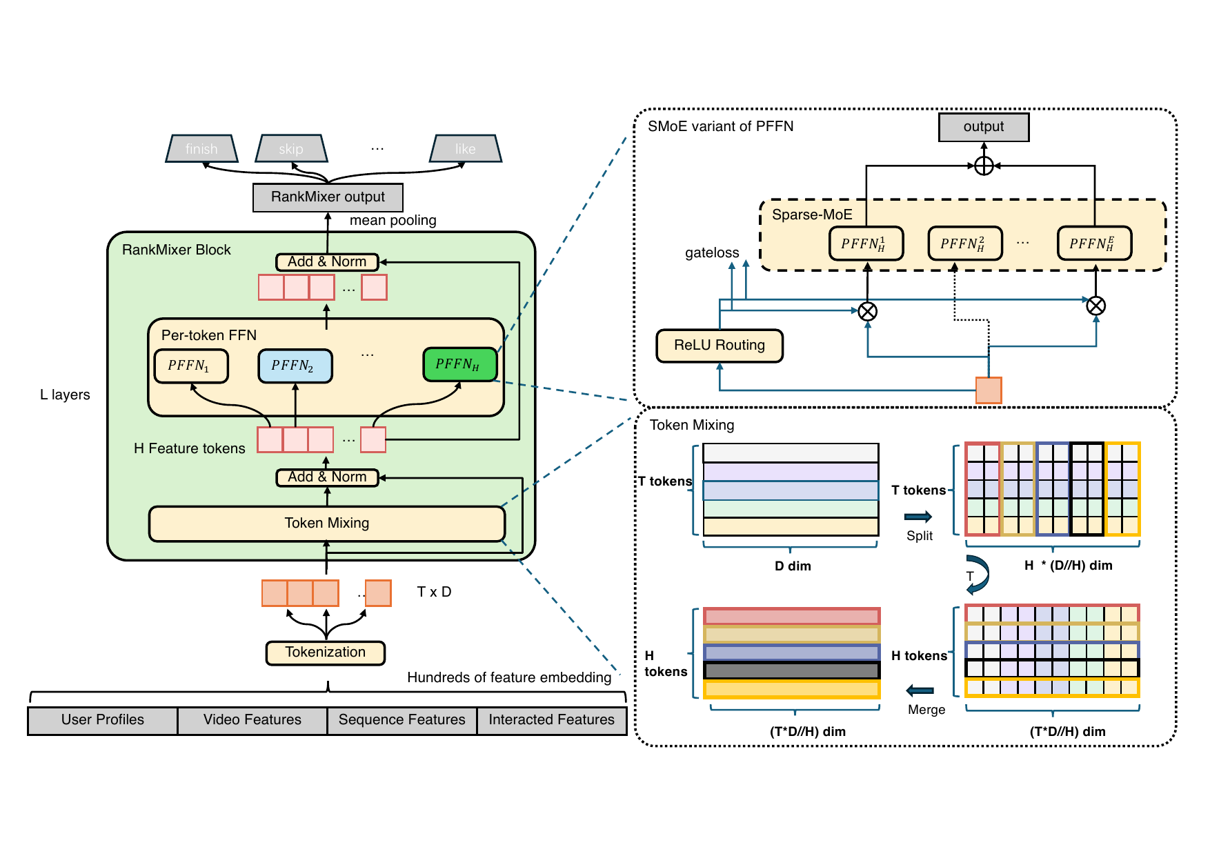
Figure 1 (Zhu et al., 2025): The RankMixer block architecture. Multi-head token mixing (parameter-free permutation) interleaves head slices across tokens; the per-token FFN (PFFN) then applies token-specific MLP transformations. The optional SMoE extension replaces the dense PFFN at 1B+ scale.
This problem verifies the 1B parameter target from the paper’s scaling formula.
Prerequisites: Per-Token Feed-Forward Network (PFFN)
The paper reports the 1B model uses \(D = 1536\), \(T = 32\), \(L = 2\), expansion factor \(k = 2\). Use the formula \(\#\text{Param} \approx 2kLTD^2\) to estimate the total dense parameter count. Compare to the reported 1B figure and explain any discrepancy.
Key insight: The formula captures only PFFN parameters; the embedding table dominates total model parameters but is excluded from the dense param count.
Sketch: \(\#\text{Dense Param} = 2 \times 2 \times 2 \times 32 \times 1536^2 \approx 0.6\text{B}\). With per-token output projection layers, plus layer norm and bias terms, the total grows to ~1B. The formula ignores the tokenization projection \(\text{Proj}(\cdot)\), input/output MLP weights, and bias terms.
3. Hardware Efficiency Analysis
⚡ The central claim of RankMixer is a 10× MFU improvement over the DLRM baseline.
3.1 Arithmetic Intensity of Self-Attention
It is tempting to assume that attention is inefficient simply because it has \(O(T^2)\) complexity, or because of the heterogeneous feature problem discussed in §1.4. The real explanation is more precise and more instructive.
A full attention block contains several distinct operations. They do not all have the same arithmetic intensity:
| Operation | What gets loaded | \(I\) | Regime |
|---|---|---|---|
| \(Q = XW_Q\), \(K = XW_K\), \(V = XW_V\) | weights \(W \in \mathbb{R}^{D \times D}\) (shared across batch) | \(\sim B\) | compute-bound ✓ |
| \(A = QK^\top / \sqrt{D/H}\) | activations \(Q, K\) (different per sample) | \(\sim 12\) | memory-bound ✗ |
| \(\text{softmax}(A)\) | activations \(A\) | \(\ll 1\) | memory-bound ✗ |
| \(\text{softmax}(A) \cdot V\) | activations \(A, V\) (different per sample) | \(\sim 12\) | memory-bound ✗ |
| output projection \(W_O\) | weights (shared across batch) | \(\sim B\) | compute-bound ✓ |
The projection GEMMs are efficient for exactly the same reason as RankMixer’s PFFN: the weight matrices are parameters shared across all \(B\) samples in the batch, so memory traffic for weights is \(O(D^2)\) independent of \(B\), giving \(I = B\). These steps are not the problem.
The problem is the attention score computation \(QK^\top\) and the weighted sum \(AV\). These are different in kind: both operands are activations, not parameters. They are distinct for every sample in the batch.
Definition (Activation-to-activation GEMM). A GEMM of the form \(C = AB\) where \(A\) and \(B\) are both activation tensors (i.e., outputs of prior layers, different per sample) has arithmetic intensity independent of batch size.
To see why, account for batch size \(B\) explicitly:
\[I_{QK^\top} = \frac{B \cdot 2T^2 D}{B \cdot 2 \times (2TD + HT^2)} = \frac{2T^2 D}{2 \times (2TD + HT^2)}\]
The \(B\) cancels. Both FLOPs and memory traffic scale linearly with \(B\), so the ratio is constant. For \(T = 32\), \(D = 1536\), \(H = 32\) (FP16, 2 bytes/element):
\[I_{QK^\top} = \frac{2 \times 1024 \times 1536}{2 \times (2 \times 32 \times 1536 + 32 \times 1024)} \approx 12 \text{ FLOPs/byte}\]
Surprisingly, this is far below the A100 ridge point of \(I^* \approx 156\) FLOPs/byte, placing the attention score kernel firmly in the memory-bandwidth-bound regime — regardless of batch size.
One might ask: if the projection GEMMs (\(W_Q, W_K, W_V, W_O\)) are efficient and the attention scores are the bottleneck, would removing the projections and using parameter-free attention (setting \(Q = K = V = X\) directly) improve MFU? No — the bottleneck is the \(QK^\top\) computation itself, not the projections. The projections were the compute-bound part. Removing them saves some efficient FLOPs while leaving the memory-bound bottleneck (\(QK^\top\), softmax, \(AV\)) fully intact. Parameter-free attention has lower MFU than full attention because the efficient operations are gone while the inefficient ones remain.
Reason 1: \(I_{QK^\top}\) scales with \(T\), and LLMs operate at large \(T\).
Simplifying the formula:
\[I_{QK^\top} = \frac{T^2D}{2TD + HT^2} = \frac{TD}{2D + HT}\]
Two limiting regimes emerge depending on whether \(HT \ll 2D\) or \(HT \gg 2D\):
\[I_{QK^\top} \approx \begin{cases} T/2 & T \ll 2D/H \quad \text{(small-}T\text{ regime)} \\ D/H & T \gg 2D/H \quad \text{(large-}T\text{ regime)} \end{cases}\]
The crossover happens at \(T^* = 2D/H\) (the head dimension doubled). For recommendation (\(D=1536\), \(H=32\)): \(T^* = 96\). Recommendation uses \(T=32 \ll 96\), so \(I \approx T/2 = 16\) — deeply in the memory-bound regime, with no escape. For a standard LLM (\(D=4096\), \(H=32\)): \(T^* = 256\). LLM training uses \(T=2048 \gg 256\), so \(I \approx D/H = 128\) — close to the A100 ridge point of 156, and approaching compute-bound for longer contexts.
| Setting | \(T\) | \(D/H\) | \(T^*\) | Regime | \(I_{QK^\top}\) |
|---|---|---|---|---|---|
| Recommendation (RankMixer target) | 32 | 48 | 96 | small-\(T\) (\(T \ll T^*\)) | ≈ 16 |
| LLM training, \(T=2048\) | 2048 | 128 | 256 | large-\(T\) (\(T \gg T^*\)) | ≈ 114 |
| LLM training, \(T=8192\) | 8192 | 128 | 256 | large-\(T\) | ≈ 200+ |
Recommendation is structurally locked in the small-\(T\) regime — there is no business case for using more than ~32 semantic feature groups, so \(T\) cannot be grown to escape the memory-bound floor.
Reason 2: In LLMs, \(QK^\top\) is a small fraction of total FLOPs.
Even when \(I_{QK^\top} < I^*\), if the memory-bound operations represent a small fraction of total FLOPs, the overall model MFU can still be high. For a standard Transformer layer at \(T=2048\), \(D=4096\):
| Operation | FLOPs | Regime |
|---|---|---|
| QKV projections + output | \(\approx 4 \times 2TD^2 = 268\text{B}\) | compute-bound |
| FFN (4× expansion) | \(\approx 2 \times 2T \times 4D^2 = 537\text{B}\) | compute-bound |
| \(QK^\top\) + \(AV\) | \(\approx 2 \times 2T^2D = 68\text{B}\) | memory-bound |
The memory-bound operations represent only \(68 / (268 + 537 + 68) \approx 8\%\) of total FLOPs. The 92% in compute-bound GEMMs dominate the wall-clock time, so the overall MFU is high even though one step is memory-bound. In recommendation with DLRM, the situation is inverted: embedding lookups, small cross-network layers, and irregular ops represent the majority of time, with few large efficient GEMMs to dilute them.
Corollary: LLM inference (autoregressive decoding) is also memory-bound.
During autoregressive generation, each decoding step produces one new token, making the effective query a single vector: \(q \in \mathbb{R}^{D/H}\) attending over the entire KV cache \(K \in \mathbb{R}^{T_{\text{ctx}} \times D/H}\). The “QK^T” becomes a matrix-vector product with \(I \approx 1\) — deeply memory-bound. This is why LLM serving has much lower MFU than LLM training, and why KV cache quantization, continuous batching, and speculative decoding exist.
3.2 Arithmetic Intensity of Token Mixing and PFFN
Token mixing is a parameter-free data permutation — it touches each byte exactly once and performs no arithmetic. Its arithmetic intensity is 0 FLOPs/byte. The entire computation in a RankMixer block therefore comes from the PFFN.
For the PFFN upward projection applied to a batch of \(B\) samples:
- FLOPs: \(B \times T \times 2D \times kD = 2BkTD^2\)
- Memory traffic (weights, assuming activations in SRAM): \(2kTD^2\) bytes
\[I_{\text{PFFN}} = \frac{2BkTD^2}{2kTD^2} = B\]
For batch size \(B = 1024\), arithmetic intensity \(= 1024\) FLOPs/byte, far above the ridge point of \(\approx 156\). The PFFN is deeply compute-bound.
For a matrix multiplication \(Y = XW\) where \(X \in \mathbb{R}^{B \times K}\) is an activation (varies per sample) and \(W \in \mathbb{R}^{K \times N}\) is a weight (fixed), FLOPs \(= 2BKN\) and weight bytes \(= 2KN\), giving \(I = B\). Batch size directly controls whether the operation is memory-bound (\(B < I^*\)) or compute-bound (\(B > I^*\)). This is why small-batch inference is memory-bound even for large models — see Memory-Bound Inference.
The general principle, unifying §3.1 and §3.2:
This distinction explains the entire MFU story:
| GEMM type | Operands | \(I\) scales with | Example |
|---|---|---|---|
| Parameter-to-activation | one fixed weight, one activation | \(B\) (batch size) | PFFN, \(XW_Q\) projections |
| Activation-to-activation | two activations, both per-sample | constant (independent of \(B\)) | \(QK^\top\), \(AV\), FM dot products |
Any cross-token interaction expressed as a dot product between two activation tensors — attention scores, factorization machine inner products, DCN cross layers — will have arithmetic intensity independent of \(B\), and will therefore be memory-bound for any batch size at small \(T\).
RankMixer eliminates all activation-to-activation computation. The cross-token interaction (token mixing) is a zero-FLOP data permutation — not a GEMM at all. The attention matrix \(A \in \mathbb{R}^{B \times H \times T \times T}\), which must be written to and read from HBM in standard attention, is never materialized. All arithmetic is in the PFFN, which is a parameter-to-activation GEMM with \(I = B\).
| Token mixing | Attention score \(QK^\top\) | |
|---|---|---|
| FLOPs | 0 | \(2BT^2D\) |
| New HBM bytes written | \(2BTD\) (permuted copy) | \(2BHT^2\) (attention matrix) |
| Intermediate tensor | none | \(A \in \mathbb{R}^{B \times H \times T \times T}\) |
| \(I\) | 0 (pure data move) | \(\sim 12\) (memory-bound, independent of \(B\)) |
3.3 MFU Measurement and Serving Cost Decomposition
| Model | Dense Params | FLOPs/Batch | GFLOPs/Param(M) | MFU | Latency |
|---|---|---|---|---|---|
| Base DLRM-8.7M | 8.7M | 52G | 5.9 | 4.51% | 16.12 ms |
| Wukong (\(l=8\), \(nL=32\)) | 122M | 442G | 3.6 | 18.51% | 33.7 ms |
| RankMixer-1B | 1B | 2,106G | 2.1 | 44.57% | 14.3 ms |
The 100× parameter increase from DLRM to RankMixer translates to only a 3% latency decrease. Two factors multiply: (1) FLOPs/Param ratio is 2.8× lower (fewer FLOPs per parameter), and (2) MFU is 9.9× higher (each FLOP is more productive). Together they nearly cancel the raw FLOPs increase, leaving latency nearly unchanged despite 100× more parameters.
3.4 Engineering Optimizations
Three system-level techniques further reduce inference latency for the deployed 1B model:
- Per-token FFN operator fusion — multiple PFFN computations merged into a single 3D tensor operation: +30% throughput.
- Mixed-precision inference (FP16) — matrix multiplications use FP16; LayerNorm uses FP32: +45% throughput, −31.5% latency.
- Sparse-GEMM acceleration — custom sparse-GEMM for the SMoE variant (§5): −40% latency.
This problem reconstructs how RankMixer-1B serves at 14.3 ms despite 115× more parameters than the 8.7M baseline.
Prerequisites: MFU Measurement and Serving Cost Decomposition
Suppose latency is proportional to \(\text{FLOPs} / (\text{MFU} \times \Pi_{\text{HW}})\). Using the numbers from §3.3, verify that the ratio \(\text{Latency}_{\text{RankMixer}} / \text{Latency}_{\text{DLRM}}\) is approximately correct. Then identify which factor — FLOPs reduction or MFU improvement — contributes more to latency parity.
Key insight: The latency ratio is \((\text{FLOPs}_{\text{RM}} / \text{MFU}_{\text{RM}}) / (\text{FLOPs}_{\text{DLRM}} / \text{MFU}_{\text{DLRM}})\).
Sketch: Ratio \(= (2106 / 0.4457) / (52 / 0.0451) = 4726 / 1153 \approx 4.1\). But the measured ratio is \(14.3 / 16.12 \approx 0.89\) — RankMixer is faster. The ~4.6× discrepancy is explained by the engineering optimizations (§3.4) applied to the deployed model. Of the two factors: MFU improvement contributes \(\approx 9.9\times\) and FLOPs increase contributes \(\approx 40.5\times\) in the wrong direction. MFU improvement (\(\approx 10\times\)) more than offsets the FLOPs increase — the gap is closed by engineering optimizations.
4. Scaling Experiments
📈
4.1 Offline Baselines at 100M Parameters
Experiments use Douyin’s production training data over a two-week window, with 300+ input features. An improvement of 0.01% AUC is considered confidently significant at production scale.
| Model | Finish AUC gain | Finish UAUC gain | Skip AUC gain | Dense Params | FLOPs/Batch |
|---|---|---|---|---|---|
| DLRM-MLP (base) | 0.0 | 0.0 | 0.0 | 8.7M | 52G |
| DLRM-MLP-100M | +0.15% | — | +0.15% | 95M | 185G |
| DCN V2 | +0.13% | +0.13% | +0.15% | 22M | 170G |
| DHEN | +0.18% | +0.26% | +0.36% | 22M | 158G |
| HiFormer | +0.48% | — | — | 116M | 326G |
| Wukong | +0.29% | +0.29% | +0.49% | 122M | 442G |
| RankMixer-100M | +0.64% | +0.72% | +0.86% | 107M | 233G |
| RankMixer-1B | +0.95% | +1.22% | +1.25% | 1B | 2,106G |
RankMixer-100M outperforms every baseline including Wukong while using 47% fewer FLOPs per batch. Scaling to 1B adds a further +0.31% Finish AUC with a 9× FLOPs increase.
4.2 Scaling Law Curves
The paper plots Finish AUC gain as a function of both parameter count and FLOPs across five architectures. Key observations:
- RankMixer exhibits the steepest slope on both the AUC vs parameters and AUC vs FLOPs curves.
- Wukong’s parameter-curve slope is steep but its FLOPs-curve slope is gentler.
- DHEN shows non-ideal scaling, reflecting limited scalability of cross-structure stacking.
The steepness of RankMixer’s scaling curve is the primary architectural claim: for a given parameter or FLOPs budget, RankMixer extracts more AUC gain than any alternative tested.
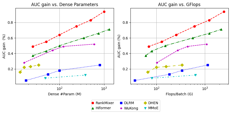
Figure 2 (Zhu et al., 2025): Scaling laws comparing Finish AUC gain vs parameter count (left) and FLOPs (right) across DLRM-MLP, DCN V2, DHEN, Wukong, and RankMixer. RankMixer exhibits the steepest slope on both axes. The x-axis is logarithmic.
4.3 Optimal Scaling Directions
RankMixer scales along four orthogonal axes: token count \(T\), hidden dimension \(D\), number of layers \(L\), and number of MoE experts \(E\). The paper finds:
- Model quality correlates primarily with total parameter count; different \((T, D, L)\) combinations achieving the same total reach nearly identical AUC.
- Increasing \(D\) (wider) is preferable to increasing \(L\) (deeper): wider \(D\) generates larger GEMM shapes, achieving higher MFU.
Final configurations chosen: - RankMixer-100M: \(D = 768\), \(T = 16\), \(L = 2\) - RankMixer-1B: \(D = 1536\), \(T = 32\), \(L = 2\)
\(L = 2\) blocks may seem surprisingly shallow for a 1B-parameter model. Because each block already has \(T\) separate MLP heads each of width \(D \times kD\), each block already has \(O(TD^2)\) parameters. Adding more blocks would inflate FLOPs without further MFU improvement. Part II (TokenMixer-Large, §9) addresses why naive depth scaling fails and how the Mixing-and-Reverting operation fixes it.
5. Sparse MoE Variant
⚙️ Scaling RankMixer beyond 1B parameters while maintaining fixed inference latency requires a Sparse Mixture-of-Experts (SMoE) extension that decouples parameter count from active FLOPs.
5.1 Motivation: Two Failure Modes of Vanilla MoE in RankMixer
Standard sparse MoE (Switch Transformer style with top-\(k\) + softmax gating) degrades markedly when naively applied to RankMixer’s PFFN:
Uniform routing ignores token information content. Different feature tokens carry different amounts of information — a rich user behavior sequence token conveys far more signal than a sparse cross-feature token. Top-\(k\) routing allocates the same number of expert activations to every token regardless, wasting capacity on low-information tokens.
Expert under-training from token-count explosion. PFFN already multiplies parameter count by \(T\). Adding \(N_e\) non-shared experts multiplies further: total experts becomes \(T \times N_e\). With a fixed routing budget of \(k\) experts per token, most experts receive very few gradient updates, leading to expert starvation.
5.2 ReLU Routing
Definition (ReLU Routing). Let \(h(\cdot) : \mathbb{R}^D \to \mathbb{R}^{N_e}\) be a learned router (linear layer). For token \(s_i\) and expert \(j\), the gate value is:
\[G_{i,j} = \text{ReLU}\!\left(h(s_i)_j\right) \geq 0\]
The aggregated output for token \(s_i\) is:
\[v_i = \sum_{j=1}^{N_e} G_{i,j} \cdot e_{i,j}(s_i)\]
Unlike softmax + top-\(k\), ReLU routing allows a variable number of experts to activate per token. Sparsity level is steered via a regularization loss:
\[\mathcal{L} = \mathcal{L}_{\text{task}} + \lambda \mathcal{L}_{\text{reg}}, \qquad \mathcal{L}_{\text{reg}} = \sum_{i=1}^{N_t} \sum_{j=1}^{N_e} G_{i,j}\]
The \(\ell_1\) penalty on gate values directly penalizes the total number of active expert slots, adaptively controlling the average activation ratio without fixing it per-token.
Softmax assigns gate weights summing to 1 — forcing competition among experts even when no expert is needed. ReLU treats each expert independently: gate \(j\) fires only if the router output is positive. This allows the degenerate case (all gates zero) for uninformative tokens, and dense activation for highly informative ones.
5.3 Dense-Training Sparse-Inference (DTSI-MoE)
Definition (DTSI-MoE). Two router functions \(h_{\text{train}}\) and \(h_{\text{infer}}\) are both updated during training. The regularization loss \(\mathcal{L}_{\text{reg}}\) is applied only to \(h_{\text{infer}}\):
- \(h_{\text{train}}\): unregularized, tends toward dense activation, providing broad gradient coverage to all experts.
- \(h_{\text{infer}}\): regularized via \(\mathcal{L}_{\text{reg}}\), tends toward sparse activation, enabling fast inference.
At inference, only \(h_{\text{infer}}\) is used. The experts are trained on dense gradient signals but evaluated under sparse routing, preventing the “dying expert” failure where sparsity at training time starves most experts.
DTSI-MoE is structurally analogous to knowledge distillation: \(h_{\text{train}}\) plays the role of a dense “teacher” ensuring all experts are well-trained, while \(h_{\text{infer}}\) is a sparse “student” that learns to approximate with fewer active experts. Unlike standard distillation, both are trained jointly end-to-end.
5.4 Scalability Results
- Vanilla SMoE (top-k): AUC degrades monotonically as sparsity increases.
- Vanilla SMoE + load-balancing loss: Some recovery, but still substantially below dense.
- DTSI + ReLU routing: Near-flat AUC curve from full activation down to 1/8 sparsity.
RankMixer with DTSI + ReLU routing scales to 8× sparsity with nearly no AUC loss and a +50% throughput improvement, validating the approach as a practical path to 10B+ parameters without proportional cost increase.
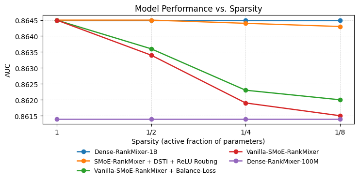
Figure 3 (Zhu et al., 2025): AUC performance of RankMixer variants at decreasing expert activation ratios (1, 1/2, 1/4, 1/8). Dense-training + ReLU-routed SMoE (DTSI-MoE) preserves near-full accuracy of the 1B dense model across all sparsity levels, while vanilla top-k MoE degrades monotonically.
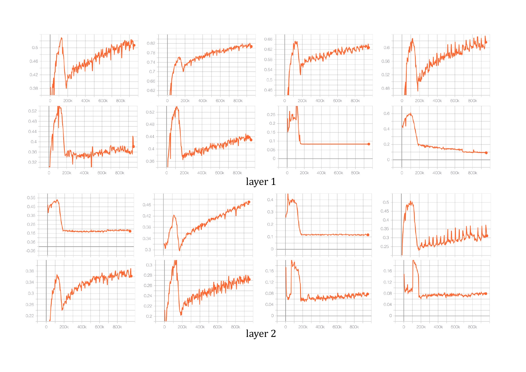
Figure 4 (Zhu et al., 2025): Activated expert ratio for different token positions in RankMixer. ReLU routing produces adaptive, token-dependent activation patterns — information-rich tokens activate more experts than sparse or low-signal tokens, naturally allocating capacity where it is most needed.
This problem derives the expected expert activation rate as a function of the regularization coefficient lambda.
Prerequisites: ReLU Routing
Assume the pre-ReLU router output \(h(s_i) \in \mathbb{R}^{N_e}\) has components drawn i.i.d. from \(\mathcal{N}(0, \sigma^2)\) at initialization. (a) Compute the expected fraction of active gates per token as a function of \(\sigma\). (b) Explain qualitatively how the \(\ell_1\) penalty \(\lambda \mathcal{L}_{\text{reg}}\) shifts this fraction during training. (c) If the target inference budget is \(k/N_e\) active experts per token, what property of \(\lambda\) ensures convergence to this budget?
Key insight: At initialization, ReLU fires on the positive half of a Gaussian, so 50% of gates are active regardless of \(\sigma\). The \(\ell_1\) penalty must push this below the target budget.
Sketch: (a) \(\mathbb{P}[G_{i,j} > 0] = \mathbb{P}[\mathcal{N}(0,\sigma^2) > 0] = 0.5\) — exactly half experts active at init. (b) The gradient of \(\mathcal{L}_{\text{reg}}\) w.r.t. the router output is \(+1\) for each active gate; this shifts the distribution of \(h(s_i)\) downward during training, reducing the fraction of positive outputs. (c) \(\lambda\) is tuned by sweeping and checking the empirical activation ratio — a fixed \(\lambda\) causes the distribution mean to drift until the \(\ell_1\) gradient is balanced by the task gradient.
6. Online A/B Results — RankMixer
🚀 RankMixer-1B was deployed for full production traffic across Feed Recommendation, Advertising, and Search on Douyin. Experiments ran for five months.
6.1 Feed Recommendation
| Metric | Douyin Overall | Douyin Low-active | Douyin Mid-active | Douyin High-active |
|---|---|---|---|---|
| Active Days | +0.20% | +0.457% | +0.432% | +0.124% |
| Duration | +0.50% | +0.859% | +1.186% | +0.492% |
| Like | +0.29% | +0.656% | +0.678% | +0.272% |
| Finish | +1.60% | +1.752% | +1.956% | +1.313% |
Low-active users benefit disproportionately — their active day lift (0.46%) is 3.7× that of high-active users (0.12%). Larger model capacity helps most when personal history is sparse: the model draws on richer cross-feature and cross-user statistical patterns.
6.2 Advertising and Search
| Scenario | Metric | Lift |
|---|---|---|
| Advertising | ΔAUC | +0.73% |
| Advertising | Advertiser Value (ADVV) | +3.90% |
| Search | ΔAUC | +1.75% |
| Search | Query change rate | −1.00% |
The search −1.0% query change rate means users find what they want with fewer reformulations, indicating genuine relevance improvement.
7. Ablation Studies — RankMixer
🔬
Block component ablations (100M scale)
| Ablation | Finish AUC change |
|---|---|
| Remove multi-head token mixing | −0.50% |
| Per-token FFN → shared FFN | −0.31% |
| Remove skip connections | −0.07% |
| Remove layer normalization | −0.05% |
Token routing strategy comparison (100M scale)
| Routing Strategy | Finish AUC change | ΔParams | ΔFLOPs |
|---|---|---|---|
| All-Concat-MLP (single large MLP) | −0.18% | 0% | 0% |
| All-Share (single shared FFN) | −0.25% | 0% | 0% |
| Self-Attention | −0.03% | +16% | +71.8% |
The comparison to self-attention is particularly revealing: self-attention costs only −0.03% AUC but requires +71.8% more FLOPs. Token mixing trades a negligible 0.03% AUC for a 42% FLOPs reduction relative to self-attention.
This problem frames the ablation results as a Pareto frontier comparison.
Prerequisites: Ablation Studies — RankMixer, Hardware Efficiency Analysis
Plot (conceptually) the four configurations from the routing ablation table on a two-axis chart: x-axis = relative FLOPs (normalized to RankMixer = 1.0), y-axis = relative AUC gain. Identify which configurations are Pareto-dominated. Then define formally what it means for a model to be on the Pareto frontier in this space and verify that RankMixer lies on it.
Key insight: A point is Pareto-dominated if another point achieves both higher AUC and lower FLOPs.
Sketch: Assign RankMixer coordinates \((1.0, 1.0)\). All-Share: \((1.0, 0.75)\) — same FLOPs, lower AUC — dominated. All-Concat-MLP: \((1.0, 0.82)\) — dominated. Self-Attention: \((1.718, 0.97)\) — higher FLOPs, slightly higher AUC. Formally, model \(A\) dominates model \(B\) iff \(\text{FLOPs}_A \leq \text{FLOPs}_B\) and \(\text{AUC}_A \geq \text{AUC}_B\) with at least one strict inequality. Self-Attention is not dominated by RankMixer but is also not the unique Pareto optimum. RankMixer lies on the Pareto frontier: no other tested configuration achieves its combination of AUC gain and FLOPs level.
8. Discussion and Limitations — RankMixer
💬
Architectural unification. The core thesis is that a single well-designed block — parameter-free token mixing followed by per-token FFN — subsumes the functionality of an entire zoo of handcrafted interaction modules (DCN, AutoInt, DHEN, FM-based approaches).
Hardware-aware design philosophy. The design choices are explicitly reverse-engineered from GPU arithmetic intensity requirements: large GEMMs, parameter-free permutations for cross-token interaction, and batch-size-amplified FLOPs-per-byte.
Limitations:
Residual dimension mismatch. The token mixing operation changes the layout of the token matrix (from \(\mathbb{R}^{T \times D}\) to \(\mathbb{R}^{H \times (T \cdot D/H)}\)), creating an impedance mismatch for inter-block residuals at large depths. The paper uses only \(L = 2\) blocks. Part II (§9) addresses this.
No head count (\(H\)) ablation. The paper sets \(H = T\) throughout but provides no sensitivity analysis.
Retrieval stage unexplored. All results pertain to re-ranking (scoring shortlisted candidates). Whether the architecture transfers to embedding-based retrieval is not addressed.
Single-task framing. Multi-task optimization challenges that arise at scale are not discussed.
Part II: TokenMixer-Large (2026)
9. Why Scale Beyond 1B: The Three Failure Modes
🏛️ TokenMixer-Large begins from a precise diagnosis of why naively scaling RankMixer past ~1B parameters fails. Three architectural failure modes are identified:
Dimension mismatch. The mixing output \(\mathbf{H} \in \mathbb{R}^{H \times (T \cdot D/H)}\) has a different layout than the input \(\mathbf{X} \in \mathbb{R}^{T \times D}\) even though they contain the same number of scalars. A reshape is required before any residual connection back to \(\mathbf{X}\), which breaks pre-norm symmetry and degrades gradient magnitude at depth.
Gradient vanishing at depth. Without skip connections spanning multiple blocks, gradients to early layers become vanishingly small as depth grows beyond ~20 blocks.
Uniform dense FFN. The per-token SwiGLU treats all tokens identically. At 7B+ parameters, this wastes capacity by forcing every expert computation to fire for every token.
TokenMixer-Large addresses each failure mode systematically: Mixing-and-Reverting for (1), inter-residual connections for (2), and Sparse Per-token MoE for (3).
10. Architecture Innovations
🏗️
10.1 Tokenization
Each raw categorical feature \(F_i\) is embedded:
\[e_i = \text{Embedding}(F_i, d_i) \in \mathbb{R}^{d_i}\]
Features are organized into \(T-1\) semantic groups \(G_0, \ldots, G_{T-2}\). Each group is projected to dimension \(D\) by a group-specific MLP:
\[X_i = \text{MLP}_i\!\bigl(\text{concat}[e_l, \ldots, e_m]\bigr) \in \mathbb{R}^D\]
A global token \(X_G\) aggregates cross-group information:
\[X_G = \text{MLP}_g\!\bigl(\text{concat}[G_1, \ldots, G_{T-1}]\bigr) \in \mathbb{R}^D\]
The full token matrix is \(\mathbf{X} = \text{concat}[X_G, X_0, \ldots, X_{T-1}] \in \mathbb{R}^{T \times D}\).
The global token plays a role analogous to the [CLS] token in BERT — it provides a summary position that accumulates cross-feature context through all subsequent mixing layers, and its output is used for the final score prediction.
Extend the RankMixer example by prepending a global token \(x_G \in \mathbb{R}^4\) computed as a small MLP over one representative vector from each semantic group:
\[x_G = \text{MLP}_g([G_{\text{user}}, G_{\text{item}}]) = [0,\, 0,\, 0,\, 0] \quad \text{(at init; will diverge during training)}\]
The full token matrix entering the block stack is now:
\[\mathbf{X} = \begin{bmatrix} 0 & 0 & 0 & 0 \\ 1 & 2 & 3 & 4 \\ 5 & 6 & 7 & 8 \end{bmatrix} \in \mathbb{R}^{3 \times 4}\]
Row 0 = global summary token; row 1 = user token; row 2 = item token. The global token starts near zero but through training accumulates a cross-feature summary used for the final score prediction. The subsequent Mix-and-Revert operations in §10.2 are demonstrated with the simpler \(T=2\) sub-example from Part I to keep the arithmetic clean.
10.2 Mixing-and-Reverting Operation
The central innovation is a two-phase symmetric transform that resolves the dimension-mismatch problem.
Definition (Mixing Phase). Given \(\mathbf{X} \in \mathbb{R}^{T \times D}\), for each head \(h\), concatenate the \(h\)-th slice from every token:
\[\text{Mix}: \quad H_h = \text{concat}[x_1^{(h)}, x_2^{(h)}, \ldots, x_T^{(h)}] \in \mathbb{R}^{T \cdot D/H}\]
Stacking gives \(\mathbf{H} = \text{stack}[H_1, \ldots, H_H] \in \mathbb{R}^{H \times (T \cdot D/H)}\). A pSwiGLU is applied in this mixed layout to produce \(\mathbf{H}' \in \mathbb{R}^{H \times (T \cdot D/H)}\).
Definition (Reverting Phase). The reverting operation is the inverse permutation of mixing: for each position \(t\), gather slice \(h\) from \(H_h'\) to reconstruct the token:
\[\text{Revert}: \quad X_t^{\text{rev}} = \text{concat}[x'^{(1)}_t, x'^{(2)}_t, \ldots, x'^{(H)}_t] \in \mathbb{R}^D\]
This yields \(\mathbf{X}^{\text{rev}} \in \mathbb{R}^{T \times D}\) — exactly the same shape as the input \(\mathbf{X}\).
Definition (TokenMixer-Large Block Output).
\[\mathbf{X}^{\text{next}} = \text{Norm}\!\bigl(\text{pSwiGLU}(\mathbf{X}^{\text{rev}}) + \mathbf{X}\bigr) \in \mathbb{R}^{T \times D}\]
The residual \(+ \mathbf{X}\) is now dimensionally consistent. Reverting is not merely a reshape — it explicitly recombines mixed-head representations back into per-token vectors, allowing the subsequent pSwiGLU to operate in the original token-feature space.
In a pre-norm transformer, the residual stream maintains a fixed shape \(\mathbb{R}^{T \times D}\) throughout all layers. The reverting step restores this invariant after each mixing operation, enabling stable pre-norm + RMSNorm stacks at 50+ layers.
Use the same \(\mathbf{X}\) from Part I. Mixing produces (as before):
\[\mathbf{H} = \text{Mix}(\mathbf{X}) = \begin{bmatrix} 1 & 2 & 5 & 6 \\ 3 & 4 & 7 & 8 \end{bmatrix} \in \mathbb{R}^{2 \times 4}\]
Row 0 of \(\mathbf{H}\) = head-0 slices from all tokens; row 1 = head-1 slices from all tokens. The pSwiGLU is applied in this head-major layout, learning transformations of each cross-token composite. Suppose pSwiGLU scales by \(0.5\) (for illustration):
\[\mathbf{H}' = \text{pSwiGLU}(\mathbf{H}) = \begin{bmatrix} 0.5 & 1 & 2.5 & 3 \\ 1.5 & 2 & 3.5 & 4 \end{bmatrix}\]
Reverting: for each token position \(t\), gather the \(t\)-th slice of size \(D/H=2\) from each row of \(\mathbf{H}'\):
\[X^{\text{rev}}_0 = \text{concat}\!\left[\underbrace{\mathbf{H}'[0,\, 0:2]}_{\text{user's h0, processed}},\; \underbrace{\mathbf{H}'[1,\, 0:2]}_{\text{user's h1, processed}}\right] = [0.5,\, 1,\, 1.5,\, 2]\]
\[X^{\text{rev}}_1 = \text{concat}\!\left[\underbrace{\mathbf{H}'[0,\, 2:4]}_{\text{item's h0, processed}},\; \underbrace{\mathbf{H}'[1,\, 2:4]}_{\text{item's h1, processed}}\right] = [2.5,\, 3,\, 3.5,\, 4]\]
\[\mathbf{X}^{\text{rev}} = \begin{bmatrix} 0.5 & 1 & 1.5 & 2 \\ 2.5 & 3 & 3.5 & 4 \end{bmatrix} \in \mathbb{R}^{2 \times 4}\]
Row 0 is now “all processed heads re-assembled for the user token”; row 1 for the item token. The residual is now semantically correct:
\[\mathbf{X}^{\text{rev}} + \mathbf{X} = \begin{bmatrix} 0.5+1 & 1+2 & 1.5+3 & 2+4 \\ 2.5+5 & 3+6 & 3.5+7 & 4+8 \end{bmatrix} = \begin{bmatrix} 1.5 & 3 & 4.5 & 6 \\ 7.5 & 9 & 10.5 & 12 \end{bmatrix}\]
Row 0 = (processed user features) + (original user features) ✓ Row 1 = (processed item features) + (original item features) ✓
Contrast with RankMixer (no reverting — adds \(\mathbf{H}'\) directly to \(\mathbf{X}\)):
\[\mathbf{H}' + \mathbf{X} = \begin{bmatrix} 0.5+1 & 1+2 & \mathbf{2.5+3} & \mathbf{3+4} \\ 1.5+5 & 2+6 & 3.5+7 & 4+8 \end{bmatrix} = \begin{bmatrix} 1.5 & 3 & \mathbf{5.5} & \mathbf{7} \\ 6.5 & 8 & 10.5 & 12 \end{bmatrix}\]
Row 0, positions 2–3: adds item’s head-0 (2.5, 3) to the user token’s second half-dimensions (3, 4) — semantically mismatched. At shallow depths (\(L=2\)) the PFFN can compensate for this scrambling; at 50+ layers the accumulated mismatch in the residual stream degrades gradient flow.
10.3 Per-Token SwiGLU
TokenMixer-Large uses per-token SwiGLU (pSwiGLU), where each token position \(t\) has its own projection matrices:
\[\text{pSwiGLU}(\cdot) = FC_{\text{down}}\!\bigl(\text{Swish}(FC_{\text{gate}}(\cdot)) \odot FC_{\text{up}}(\cdot)\bigr)\]
with token-specific projections \(FC_i(\mathbf{x}) = W_i^t x_t + b_i^t\), where \(\{W_{\text{up}}^t, W_{\text{gate}}^t\} \in \mathbb{R}^{D \times nD}\) and \(W_{\text{down}}^t \in \mathbb{R}^{nD \times D}\).
For token position \(t\) with reverted representation \(X^{\text{rev}}_t \in \mathbb{R}^D\), the pSwiGLU computes:
\[\text{pSwiGLU}(X^{\text{rev}}_t) = W_{\text{down}}^t \cdot \underbrace{\bigl(\text{Swish}(W_{\text{gate}}^t X^{\text{rev}}_t) \odot W_{\text{up}}^t X^{\text{rev}}_t\bigr)}_{\text{gated hidden state} \in \mathbb{R}^{nD}}\]
The Swish gate \(\sigma = \text{Swish}(W_{\text{gate}}^t X^{\text{rev}}_t) \in \mathbb{R}^{nD}\) is a learned, input-dependent mask: each of the \(nD\) hidden dimensions can be suppressed (near zero) or passed through (near one) based on the content of \(X^{\text{rev}}_t\). This lets each token position selectively activate different parts of its FFN capacity depending on what it received from the mixing step.
A plain per-token ReLU FFN (\(W_2^t \cdot \text{ReLU}(W_1^t X^{\text{rev}}_t)\)) has fixed sparsity from the ReLU nonlinearity but no input-dependent gating — every feature competes equally. The ablation (−0.10% for ReLU vs −0.21% for shared SwiGLU) shows that per-token weights matter more than the gating mechanism, but gating contributes an additional 0.10% on top.
Replacing pSwiGLU with a standard shared SwiGLU costs −0.21% AUC; replacing it with a per-token FFN (ReLU, no gating) costs −0.10% AUC. The per-token gating mechanism contributes more than the token-specificity alone.
10.4 Residuals and Normalization
Pre-Norm with RMSNorm throughout, consistent with modern LLM practice:
\[\text{Output} = \text{SubLayer}(\text{RMSNorm}(\mathbf{X})) + \mathbf{X}\]
10.5 Inter-Residual and Auxiliary Loss
For networks beyond ~20 blocks, standard residuals are insufficient to propagate gradients to early layers. TokenMixer-Large introduces inter-residual connections: skip connections that bypass 2–3 consecutive blocks.
Definition (Inter-Residual). Let \(\mathbf{X}^{(\ell)}\) denote the output of block \(\ell\). An inter-residual with stride \(s\) adds:
\[\mathbf{X}^{(\ell+s)} \leftarrow \mathbf{X}^{(\ell+s)} + \mathbf{X}^{(\ell)}\]
at regular intervals \(s \in \{2, 3\}\) throughout the network.
An auxiliary loss is applied at intermediate block outputs:
\[\mathcal{L}_{\text{total}} = \mathcal{L}_{\text{CE}}(y, \hat{y}^{(L)}) + \lambda \sum_{\ell \in S} \mathcal{L}_{\text{CE}}(y, \hat{y}^{(\ell)})\]
At depth 50+, the gradient of \(\mathcal{L}_{\text{CE}}\) with respect to block 5’s parameters has been attenuated by ~45 Jacobian multiplications. The auxiliary loss at block \(\ell\) provides a direct gradient signal to all blocks \(\leq \ell\), bypassing the deep chain. This is analogous to GoogLeNet’s auxiliary classifiers.
Ablation: removing both inter-residuals and auxiliary loss costs −0.04% AUC at the 4B scale; removing the standard within-block residual costs −0.15% AUC.
Figure 5 (Jiang et al., 2026): Inter-residual connections and auxiliary loss in TokenMixer-Large. Skip connections with stride \(s \in \{2, 3\}\) bypass groups of consecutive blocks, and auxiliary cross-entropy losses at intermediate layers provide direct gradient signals to early blocks — essential for stable training at 50+ block depth.
With \(s=2\), every other block’s output is added to the block two steps ahead. Tracing the signal path for a single token vector:
X^(0) ──► Block 1 ──► X^(1) ──► Block 2 ──► X^(2)
   └──────────────── (+) ──────────────────►  X^(2) += X^(0)

X^(2) ──► Block 3 ──► X^(3) ──► Block 4 ──► X^(4)
   └──────────────── (+) ──────────────────►  X^(4) += X^(2)
Without inter-residuals, a gradient flowing back to block 1 must pass through Jacobians for blocks 2, 3, and 4 — four multiplications that can each attenuate it. With stride-2 inter-residuals, the gradient from block 3’s loss also has a direct path back to block 1 (bypassing block 2), and the auxiliary loss at block 2 directly supervises blocks 1 and 2. At 50 blocks the difference between chaining 50 Jacobians and having skip connections every 2 steps is the difference between stable and vanishing gradients.
| Step | Tensor shape | Semantic meaning of each row |
|---|---|---|
| Input \(\mathbf{X}\) | \((T, D)\) | Each row = one feature group (global, user, item, …) |
| After Mix | \((T, D)\) | Each row = one head-slice gathered across all groups |
| After pSwiGLU (in mixed layout) | \((T, D)\) | Each row = gated transformation of cross-token composite |
| After Revert | \((T, D)\) | Each row = processed heads re-assembled per token (shape-consistent with input) |
| After residual \(+ \mathbf{X}\) and RMSNorm | \((T, D)\) | Each row = token-specific representation enriched by cross-token context |
| After second pSwiGLU + residual | \((T, D)\) | Block output: same shape, ready for next block or pooling |
The Revert step is the key difference from RankMixer: it restores the token-major semantics of each row before the residual addition, enabling semantically correct skip connections at any depth.
10.6 Block Architecture Diagram
flowchart TD
    X["X in R^{TxD}
input tokens"] --> RN1["RMSNorm"]
    RN1 --> MIX["Mixing Phase
split heads, concat across tokens
H in R^{Hx(T D/H)}"]
    MIX --> SWIGLU1["pSwiGLU
(in mixed layout)"]
    SWIGLU1 --> REV["Reverting Phase
gather heads to per-token
X^rev in R^{TxD}"]
    REV --> ADD1["+ residual X"]
    ADD1 --> RN2["RMSNorm"]
    RN2 --> SWIGLU2["Per-token SwiGLU
token-specific W^t"]
    SWIGLU2 --> ADD2["+ residual"]
    ADD2 --> OUT["X^next in R^{TxD}"]
    X -.->|"inter-residual
every s=2-3 blocks"| SKIP["downstream block"]
    OUT --> SKIP
Figure 6 (Jiang et al., 2026): The TokenMixer-Large block architecture. Each block consists of (RMSNorm → Mixing → SP-MoE → Reverting → RMSNorm → SP-MoE) with inner and inter-block residuals. The Reverting phase restores the token-major layout after mixing, enabling dimensionally consistent residuals at any depth. SP-MoE replaces the dense pSwiGLU at 7B–15B scale.
This problem makes precise that mixing-and-reverting is an exact permutation, not a learned projection.
Prerequisites: Mixing-and-Reverting Operation
Let \(\mathbf{X} \in \mathbb{R}^{T \times D}\) with \(H\) heads. Write the mixing operation \(\mathbf{H} = \text{Mix}(\mathbf{X})\) explicitly as a matrix multiplication \(\mathbf{H} = P \cdot \text{vec}(\mathbf{X})\) for a permutation matrix \(P\). Then show that the reverting operation satisfies \(\text{Revert}(\mathbf{H}) = P^\top \mathbf{H}\). Conclude that \(\text{Revert}(\text{Mix}(\mathbf{X})) = \mathbf{X}\) exactly — there is no information loss.
Key insight: Mixing concatenates the \(h\)-th head slice of each token; reverting interleaves them back. Both are index permutations on the flattened vector \(\text{vec}(\mathbf{X})\).
Sketch: Index \((t, d)\) in \(\mathbf{X}\) maps to head \(h = \lfloor d \cdot H / D \rfloor\) and within-head position \(d' = d \bmod (D/H)\). In \(\mathbf{H}\), this scalar lives at position \((h, t \cdot D/H + d')\). This is a bijection on \(\{1, \ldots, TD\}\), hence a permutation matrix \(P\). The reverting applies \(P^{-1} = P^\top\) (permutation matrices are orthogonal). Therefore \(P^\top P \cdot \text{vec}(\mathbf{X}) = \text{vec}(\mathbf{X})\).
11. Sparse Per-Token MoE
⚡ At 7B–15B parameters, it becomes infeasible to activate all parameters for every token at every layer. TokenMixer-Large introduces Sparse Per-token MoE (SP-MoE).
11.1 Formulation
Let there be \(E\) experts, each a scaled-down pSwiGLU. For token \(x_t\), a gating network selects the top-\(k\) experts:
\[\text{SP-MoE}(x_t) = \sum_{j=1}^{k} g_j(x_t) \cdot \text{Expert}_j(x_t)\]
where \(g_j(x_t) = \text{softmax}(\text{top-}k(W_g x_t))_j\). Each expert has width \(nD/E\), so that each expert is \(1/E\) the width of the corresponding dense pSwiGLU.
Per-token routing means each token independently selects its \(k\) experts. This contrasts with sequence-level MoE (Switch Transformer), which routes entire sequence positions identically — suboptimal for ranking where different semantic token groups (user vs. item vs. context) should leverage different experts.
Switch Transformer uses top-1 routing with a capacity factor \(C\) that hard-caps how many tokens each expert can process. SP-MoE uses top-\(k\) with \(k \geq 2\) and a shared expert, and does not apply a hard capacity cap (sequence length \(T\) is small enough that capacity constraints are less severe).
11.2 First Enlarge, Then Sparsify
The strategy is sparse train, sparse infer — sparsity is fixed at training time so inference requires no special conversion. For a \(1:2\) sparsity model, active FLOPs drop by approximately \(2\times\) while parameter count doubles relative to a single-expert baseline.
Figure 7 (Jiang et al., 2026): “First Enlarge, Then Sparsify” illustration. Starting from a dense baseline, the model is first enlarged by adding experts (increasing total parameters), then sparsified so only a fraction of experts activate per token at inference. This sequence — train sparse from the start — avoids the dense-to-sparse conversion gap that degrades accuracy in post-hoc pruning.
TokenMixer-Large 4B dense: 29.8T FLOPs/batch. TokenMixer-Large 4B SP-MoE (2.3B active, \(1:2\) sparsity): 15.1T FLOPs/batch. AUC: both achieve +1.14% vs the 500M baseline. The SP-MoE halves inference cost with no AUC penalty.
11.3 Shared Expert
One expert is always active, regardless of gating:
\[\text{SP-MoE}(x_t) = \sum_{i=1}^{k-1} g_i(x_t) \cdot \text{Expert}_i(x_t) + \text{SharedExpert}(x_t)\]
The shared expert acts as a “default path” ensuring all tokens receive at least one full transformation, preventing catastrophic forgetting of common patterns when the router is uncertain. Removing it costs −0.02% AUC.
Figure 9 (Jiang et al., 2026): SP-MoE expert activation load balance at 1:2 sparsity. Each bar shows the fraction of tokens routed to each expert across the sequence. The distribution is approximately uniform, confirming that the auxiliary load-balancing loss prevents expert collapse even under per-token routing.
11.4 Gate Value Scaling
A scalar \(\alpha\) is applied to the gated sum, set inversely proportional to the sparsity ratio: \(\alpha = 2\) for \(1:2\) sparsity, \(\alpha = 4\) for \(1:4\) sparsity. Without this correction, the softmax gate values sum to 1 over \(k-1\) selected experts, so the magnitude of the routed contribution decreases as \(k\) shrinks. Removing \(\alpha\) costs −0.03% AUC.
11.5 Down-Matrix Small Initialization
The down-projection matrix \(W_{\text{down}}^{t,j}\) of each expert pSwiGLU is initialized with standard deviation \(0.01\) (vs. default \(1.0\)). This forces expert outputs near-zero at initialization, so the model starts close to a passthrough and learns expert specialization gradually. This is analogous to small-init residual branches in NTK theory. Removing it costs −0.03% AUC.
This problem derives why uniform routing is a local optimum of the auxiliary load balancing objective.
Prerequisites: Formulation
Consider \(E\) routable experts and \(B\) tokens per batch. Define the load of expert \(j\) as \(\ell_j = \sum_{t=1}^B \mathbf{1}[\text{token } t \text{ routes to expert } j]\) and the soft routing probability \(p_j = \frac{1}{B}\sum_{t=1}^B g_j(x_t)\). The standard auxiliary loss is \(\mathcal{L}_{\text{bal}} = \alpha_{\text{bal}} \cdot E \sum_{j=1}^E \ell_j \cdot p_j\). Show that this loss is minimized when \(\ell_j = B/E\) for all \(j\), and explain why the product \(\ell_j \cdot p_j\) is a tighter surrogate than \(\ell_j^2\) for penalizing imbalance.
Key insight: The product form \(\ell_j \cdot p_j\) is differentiable in \(p_j\) (unlike \(\ell_j\), which is discrete), so its gradient can be back-propagated to the gating network.
Sketch: By AM-GM, \(\sum_j \ell_j p_j \geq E \cdot (\prod_j \ell_j p_j)^{1/E}\). When \(\sum_j \ell_j = B\) and \(\sum_j p_j = 1\), the sum \(\sum_j \ell_j p_j\) is minimized subject to these constraints when \(\ell_j = B/E\) and \(p_j = 1/E\) — any deviation creates a larger product sum. The product \(\ell_j \cdot p_j\) couples the discrete routing (\(\ell_j\)) with the differentiable gate (\(p_j\)), enabling gradient flow; \(\ell_j^2\) alone has no gradient w.r.t. the gating network parameters.
12. Scaling to 7B–15B
📈
12.1 Offline Scaling Curves
The paper fits a log-linear relationship between parameter count \(N\) and AUC gain:
\[\Delta\text{AUC}(N) \approx a \cdot \log N + b\]
Key offline results (vs. DLRM-MLP-500M baseline):
| Model | ΔAUC | Params | FLOPs/Batch |
|---|---|---|---|
| Wukong | +0.76% | 513M | 4.6T |
| RankMixer (TokenMixer) | +0.84% | 567M | 4.6T |
| TokenMixer-Large 500M | +0.94% | 501M | 4.2T |
| TokenMixer-Large 4B | +1.14% | 4.6B | 29.8T |
| TokenMixer-Large 7B | +1.20% | 7.6B | 49.0T |
| TokenMixer-Large 4B SP-MoE | +1.14% | 2.3B active | 15.1T |
A key finding: beyond 1B parameters, scaling requires balanced expansion across width \(D\), depth \(L\), and expansion factor \(n\) simultaneously — scaling any single dimension yields diminishing returns.
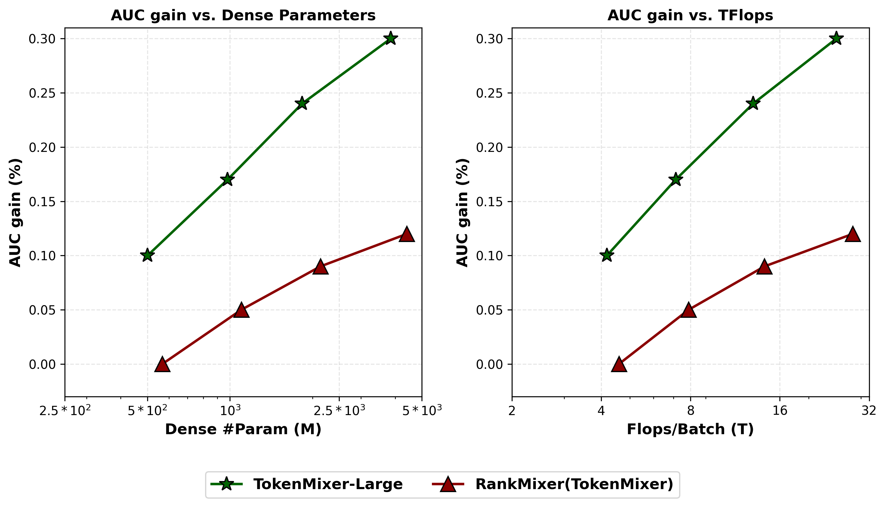
Figure 8 (Jiang et al., 2026): Scaling laws comparing AUC gain vs parameter count (left) and FLOPs (right) for Wukong, RankMixer (TokenMixer), and TokenMixer-Large across multiple Douyin scenarios (e-commerce 15B, 7B, 4B). TokenMixer-Large achieves consistent log-linear AUC improvements up to 15B parameters, with the steepest scaling slope among all tested models. The x-axis is logarithmic.
The paper further notes that DCN-style cross-network components become less valuable at larger scales:
| Params | DCN Gain |
|---|---|
| 150M | +0.09% |
| 500M | +0.04% |
| 700M | +0.00% |
This suggests the token-mixing backbone subsumes the cross-feature interaction function that DCN was designed to provide, making DCN redundant at scale.
12.2 Data Hunger at Scale
| Params | Convergence Training Days | ΔUAUC |
|---|---|---|
| 90M | 14 days | +0.94% |
| 500M | 30 days | +0.62% |
| 2.3B | 30 days | +0.41% |
| 2.3B | 60 days | +0.70% |
The 2.3B model trained for 30 days underperforms the 500M model — it simply has not seen enough data to fill its capacity. At 60 days, it recovers and exceeds the 500M baseline. Larger models require proportionally more training data, consistent with Chinchilla-style scaling laws.
12.3 DCN Diminishing Returns
The vanishing DCN gain at 700M+ parameters indicates that the cross-feature interaction capability of explicit polynomial cross networks is already captured by the depth and width of the token-mixing stack at scale. Including DCN at large scale adds FLOPs (125.8T vs 4.6T for Wukong/TokenMixer at 500M) without AUC benefit.
This problem estimates the effective scaling exponent from the offline AUC data.
Prerequisites: Offline Scaling Curves, Neural Scaling Laws
Using the three data points (TokenMixer-Large 500M: +0.94%, 4B: +1.14%, 7B: +1.20%) as \(\Delta\text{AUC}(N)\) vs \(N\) (in billions), fit a power law \(\Delta\text{AUC}(N) = c \cdot N^\alpha\) by taking logarithms. Estimate \(\alpha\). Is the observed exponent consistent with the \(\alpha \approx 0.1\) scaling exponent commonly reported for language model loss?
Key insight: The gains are compressing logarithmically, implying a small but positive exponent.
Sketch: Taking logs: \(\ln(0.94) \approx -0.062\), \(\ln(1.14) \approx 0.131\), \(\ln(1.20) \approx 0.182\); \(\ln(0.5) \approx -0.693\), \(\ln(4) \approx 1.386\), \(\ln(7) \approx 1.946\). Linear regression gives slope \(\alpha \approx (0.182 - (-0.062)) / (1.946 - (-0.693)) \approx 0.09\). This is close to the \(\alpha \approx 0.07\)–\(0.1\) range for LLM scaling. A smaller \(\alpha\) implies steeply diminishing returns — doubling parameters yields only a \(2^\alpha - 1 \approx 6\%\) relative gain in \(\Delta\text{AUC}\), justifying the focus on compute-efficient SP-MoE.
13. Training and Serving Optimizations
🔧
13.1 Custom MoE Operators
| Operator | Train Time (ms) | Train % | Serving Time (ms) | Serving % |
|---|---|---|---|---|
| MoEGroupedFFN | 136.77 | 89.18% | 7.43 | 98.35% |
| MoEPermute | 6.32 | 4.12% | 0.06 | 0.75% |
| MoEUnpermute | 10.27 | 6.69% | 0.07 | 0.90% |
The permute and unpermute operations reorder token activations so that all tokens routed to expert \(j\) are contiguous in memory before the GroupedFFN kernel executes — essential for batched matrix multiplication efficiency. The GroupedFFN dominates at both training (89%) and serving (98%), making it the target for FP8 quantization.
13.2 FP8 Quantization
The MoEGroupedFFN is quantized to FP8 (E4M3 format) for serving, providing 2× memory bandwidth reduction vs FP16 and hardware-accelerated matrix multiplication on H100 GPUs. Result: 1.7× serving speedup with negligible AUC degradation.
The GroupedFFN at serving is memory-bandwidth bound (Table 13.1). FP8 directly reduces bytes transferred per matrix multiplication, unlocking the memory bandwidth bottleneck. Compute-bound operations would benefit less.
13.3 Token Parallel Distributed Training
Token parallelism partitions the \(T\) tokens across \(P\) GPUs, keeping model parameters on each device while splitting the sequence. Each GPU processes \(T/P\) tokens; an all-reduce aggregates after the per-token FFN.
A 4-way token parallel configuration yields: - 29.2% throughput improvement (raw, without communication overlap) - 96.6% throughput improvement with communication-computation overlap - MFU improved to 60% in the advertising backbone
14. Online Experiments — TokenMixer-Large
🚀
14.1 Business Metrics
| Scenario | Model Scale | ΔAUC | Business Metric | Lift |
|---|---|---|---|---|
| Feed Ads | 15B | +0.35% | ADSS | +2.0% |
| E-Commerce | 7B | +0.51% | Orders | +1.66% |
| E-Commerce | 7B | +0.51% | Per-capita preview GMV | +2.98% |
| Live Streaming | 4B | +0.70% ΔUAUC | Pay revenue | +1.4% |
The +2.98% GMV gain on e-commerce is the headline result, representing one of the largest single-model improvements reported in recent industrial recommender papers.
14.2 Feed Recommendation Breakdown
| User Segment | Active Day Lift | Watch Duration Lift | Like Lift |
|---|---|---|---|
| Low-active | +1.74% | +3.64% | +8.16% |
| Middle-active | +0.71% | +1.53% | +2.58% |
| High-active | +0.14% | +0.63% | +1.83% |
Low-active users benefit most — ~12× vs high-active users on like rate — consistent with larger model capacity helping most when user histories are sparse.
This problem estimates the minimum detectable effect for the reported business metric lifts.
Prerequisites: Business Metrics
Suppose the e-commerce A/B test assigns 50%/50% traffic split with \(n = 10^7\) users per arm. Assume per-user GMV follows a log-normal distribution with coefficient of variation (CV = std/mean) of 2.0. Using a two-sample \(t\)-test at \(\alpha = 0.05\) two-sided, \(\beta = 0.20\) (80% power), derive the minimum detectable effect (MDE) as a percentage lift in mean GMV. Is the +2.98% GMV lift detectable at this sample size?
Key insight: The MDE for a relative lift in mean is \(\text{MDE} = (z_{\alpha/2} + z_\beta) \cdot \text{CV} / \sqrt{n/2}\).
Sketch: For \(z_{0.025} = 1.96\), \(z_{0.20} = 0.84\): \(\text{MDE} = (1.96 + 0.84) \cdot 2.0 / \sqrt{5 \times 10^6} = 2.80 \cdot 2.0 / 2236 \approx 0.25\%\). The reported +2.98% lift is approximately \(12\times\) the MDE — not borderline. At \(10^7\) users per arm and CV=2, even a 0.25% relative lift is detectable.
15. Ablation Studies — TokenMixer-Large
🔬
TokenMixer-Large Block ablations (4B scale)
| Ablation | ΔAUC |
|---|---|
| w/o Global Token | −0.02% |
| w/o Mixing and Reverting | −0.27% |
| w/o Residual | −0.15% |
| w/o Inter-Residual and AuxLoss | −0.04% |
| pSwiGLU → SwiGLU (shared) | −0.21% |
| pSwiGLU → Per-token FFN | −0.10% |
SP-MoE ablations (4B scale)
| Ablation | ΔAUC | ΔParams | ΔFLOPs |
|---|---|---|---|
| w/o Shared Expert | −0.02% | 0% | 0% |
| w/o Gate Value Scaling | −0.03% | 0% | 0% |
| w/o Down-Matrix Small Init | −0.03% | 0% | 0% |
| SP-MoE → Sparse MoE (global routing) | −0.10% | 0% | 0% |
The last row is the most informative: replacing per-token routing with global (sequence-level) MoE routing costs −0.10% AUC at zero parameter or FLOPs overhead. This confirms that per-token routing is qualitatively more expressive than global routing for the heterogeneous-feature setting of recommendation ranking.
16. Discussion and Limitations — TokenMixer-Large
💬
Pure model design. A recurring theme is the elimination of fragmented operators — ad-hoc task-specific components accumulated over years of system iteration. TokenMixer-Large argues that a single well-designed block (Mixing-and-Reverting + pSwiGLU + SP-MoE) subsumes the functionality of these operators while being easier to scale and profile.
Scaling to 15B is not free. Three practical constraints:
- Data constraint. The 2.3B model requires ≥60 days of Douyin training data to converge; scaling to 15B implies even longer horizons or faster data pipelines.
- Latency constraint. Serving a 15B model within a 10 ms SLA requires careful FP8 quantization, model parallelism, and hardware-specific kernel tuning.
- Scenario-specific saturation. The e-commerce scenario saturates at 7B; live streaming at 4B. Continued scaling should be driven by scenario-specific offline scaling laws, not a global parameter target.
Limitations:
- No retrieval-stage results. TokenMixer-Large is a ranking model; transfer to embedding-based retrieval (ANN search) is unexplored.
- Cursory load balancing analysis. Expert activation distributions are shown but routing collapse or expert specialization are not quantified.
- No ablation on head count \(H\). A critical hyperparameter for Mixing-and-Reverting, but no sensitivity analysis is provided.
References
| Reference Name | Brief Summary | Link to Reference |
|---|---|---|
| RankMixer (Zhu et al., 2025) | Primary paper: multi-head token mixing, per-token FFN, ReLU+DTSI MoE; MFU 4.5%→44.6% | https://arxiv.org/abs/2507.15551 |
| TokenMixer-Large (Jiang et al., 2026) | Follow-up: Mixing-and-Reverting, SP-MoE; scales to 7B–15B, +2.98% GMV | https://arxiv.org/abs/2602.06563 |
| MLP-Mixer (Tolstikhin et al., 2021) | Vision architecture replacing attention with token-mixing and channel-mixing MLPs; direct inspiration | https://arxiv.org/abs/2105.01601 |
| DLRM (Naumov et al., 2019) | Facebook’s deep learning recommendation model; defines the baseline architecture | https://arxiv.org/abs/1906.00091 |
| DCN V2 (Wang et al., 2021) | Deep & Cross Network V2; explicit polynomial cross-feature interactions; beaten by RankMixer-100M | https://arxiv.org/abs/2008.13535 |
| DHEN (Zhang et al., 2022) | Deep hierarchical ensemble network; strong 100M-scale baseline | https://arxiv.org/abs/2203.11014 |
| Wide & Deep (Cheng et al., 2016) | Foundational two-tower ranking model; ancestor of DLRM | https://arxiv.org/abs/1606.07792 |
| Wukong (Zhang et al., 2024) | Stacked FM and LCB blocks; closest prior-art comparison at 100M–500M scale | https://arxiv.org/abs/2403.02545 |
| Switch Transformers (Fedus et al., 2022) | Sparse MoE with top-1 routing; motivates design of DTSI-MoE and SP-MoE | https://arxiv.org/abs/2101.03961 |
| Scaling Laws for NLMs (Kaplan et al., 2020) | Power-law scaling of language model loss; framework applied to ranking AUC gains | https://arxiv.org/abs/2001.08361 |
| Chinchilla (Hoffmann et al., 2022) | Compute-optimal scaling: model size and data must scale together; directly relevant to §12.2 | https://arxiv.org/abs/2203.15556 |
| SwiGLU (Shazeer, 2020) | Gated linear unit variant used as activation in TokenMixer-Large’s FFN sub-layers | https://arxiv.org/abs/2002.05202 |