Johnson-Lindenstrauss Lemma
Table of Contents
- 1. Setup and Motivation
- 2. The Johnson-Lindenstrauss Lemma
- 3. Proof via Gaussian Projection
- 4. Inner Product Preservation
- 5. Matrix Constructions
- 6. Lower Bounds
- 7. Applications
- 8. References
1. Setup and Motivation 📐
1.1 The Curse of Dimensionality
Many computational tasks — nearest-neighbor search, clustering, regression — degrade severely as ambient dimension \(d\) grows. Storage costs scale as \(O(nd)\), distance computations take \(O(d)\) time, and geometric structures that hold in low dimensions (e.g., ball coverings with few centers) require exponentially many pieces in high dimensions. A central question in computational geometry and learning theory is: when can we reduce dimension without paying an unacceptable price in geometric fidelity?
The Johnson-Lindenstrauss lemma (JL lemma) gives a sharp, constructive answer for Euclidean geometry: any \(n\)-point cloud in \(\mathbb{R}^d\) can be linearly embedded into \(\mathbb{R}^k\) with \(k = O(\varepsilon^{-2} \log n)\) while distorting every pairwise distance by at most a factor of \((1 \pm \varepsilon)\). Crucially, the target dimension \(k\) is independent of the original dimension \(d\). 🔑
The two plots below make the bound concrete. The first shows that \(k\) grows only logarithmically in \(n\): even for \(n = 10^9\) observations with \(\varepsilon = 0.1\), fewer than \(10^4\) dimensions suffice. The second shows how rapidly \(k\) decreases as the allowed distortion \(\varepsilon\) grows — a factor-of-2 relaxation (from \(\varepsilon = 0.1\) to \(\varepsilon = 0.3\)) roughly halves the required dimension.
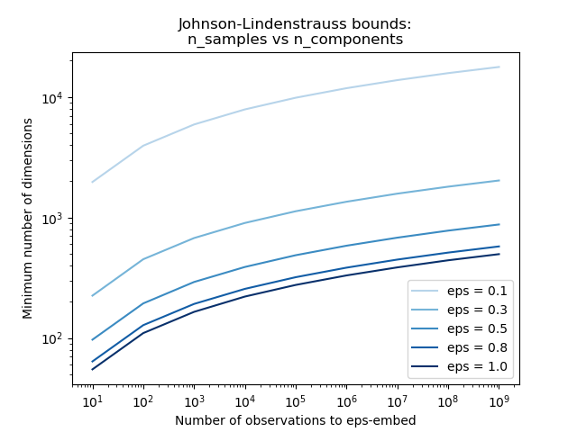 The JL bound \(k = O(\varepsilon^{-2} \log n)\) plotted on log-log axes. Each curve corresponds to a fixed distortion tolerance \(\varepsilon\). The logarithmic growth in \(n\) is the central miracle: one million data points require only ~500 dimensions at \(\varepsilon = 0.5\). (Reproduced from scikit-learn JL bounds example.)
 The same bound viewed as \(k\) versus \(\varepsilon\) on a semi-log scale. The steep drop near \(\varepsilon = 0\) reflects the \(\varepsilon^{-2}\) factor; beyond \(\varepsilon \approx 0.3\) the curves flatten. (Reproduced from scikit-learn JL bounds example.)
1.2 Notation and Problem Statement
Let \(\|\cdot\|\) denote the Euclidean norm on \(\mathbb{R}^d\). For a map \(f : \mathbb{R}^d \to \mathbb{R}^k\) and a set \(\mathcal{P} \subset \mathbb{R}^d\) with \(|\mathcal{P}| = n\), we say \(f\) is an \((1 \pm \varepsilon)\)-isometric embedding of \(\mathcal{P}\) if
\[ (1 - \varepsilon)\|u - v\|^2 \leq \|f(u) - f(v)\|^2 \leq (1 + \varepsilon)\|u - v\|^2 \quad \text{for all } u, v \in \mathcal{P}. \]
We work with squared norms throughout since that is what Gaussian projections directly control; the \((1 \pm \varepsilon)\) bound on squared distances implies a \((1 \pm \varepsilon)\)-bound on distances to first order.
Because \(f\) is linear, \(\|f(u) - f(v)\|^2 = \|f(u - v)\|^2\). It therefore suffices to prove that a single fixed unit vector \(x \in \mathbb{R}^d\) satisfies \((1-\varepsilon)\|x\|^2 \le \|f(x)\|^2 \le (1+\varepsilon)\|x\|^2\) with high enough probability; we then union-bound over all \(\binom{n}{2}\) pairs.
2. The Johnson-Lindenstrauss Lemma 🔑
2.1 Formal Statement
Theorem (Johnson-Lindenstrauss, 1984). Let \(\varepsilon \in (0, 1)\) and let \(\mathcal{P} \subset \mathbb{R}^d\) be a finite set of \(n\) points. Set
\[ k \geq \frac{4 \ln n}{\varepsilon^2 / 2 - \varepsilon^3 / 3}. \]
Then there exists a linear map \(f : \mathbb{R}^d \to \mathbb{R}^k\) such that \(f\) is a \((1 \pm \varepsilon)\)-isometric embedding of \(\mathcal{P}\). Moreover, a random Gaussian projection achieves this with positive probability (in fact, with probability at least \(1 - 1/n\)).
The denominator simplifies: for small \(\varepsilon\), \(\varepsilon^2/2 - \varepsilon^3/3 \approx \varepsilon^2/2\), giving the cleaner sufficient condition \(k = O(\varepsilon^{-2} \log n)\).
The original 1984 paper by Johnson and Lindenstrauss used a non-constructive argument (via measure theory on the sphere) to show that a random orthogonal projection works. The explicit chi-squared analysis presented here is from Dasgupta and Gupta (2003), which gave the first elementary proof.
2.2 The Distributional JL Lemma
The statement above guarantees existence of a good embedding; in practice we want to sample the embedding without seeing the data. The distributional form captures this.
Lemma (Distributional JL Lemma). For every \(d \in \mathbb{N}\), \(\varepsilon, \delta \in (0,1)\), there exists a distribution \(\mathcal{F}\) over linear maps \(f : \mathbb{R}^d \to \mathbb{R}^k\) with \(k = \Theta(\varepsilon^{-2} \log(1/\delta))\) such that for every fixed \(x \in \mathbb{R}^d\):
\[\Pr_{f \sim \mathcal{F}}\!\left[\bigl|\|f(x)\|^2 - \|x\|^2\bigr| \leq \varepsilon\|x\|^2\right] \geq 1 - \delta.\]
The JL theorem (Lemma 2.1) follows from the distributional version by setting \(\delta = 1/n^2\) and union-bounding over all \(\binom{n}{2}\) pairs of difference vectors.
The distribution \(\mathcal{F}\) depends only on \(d\), \(\varepsilon\), and \(\delta\) — not on the input vectors. This means we can sample \(f\) before seeing the data, compute the sketch in one pass over a stream, or distribute the computation across machines that each hold part of the dataset. The Gaussian JL matrix is an explicit witness to \(\mathcal{F}\).
2.3 The Core Probabilistic Lemma
The proof reduces to establishing the following one-vector concentration result.
Lemma (JL Concentration). Let \(x \in \mathbb{R}^d\) with \(\|x\| = 1\). Let \(A \in \mathbb{R}^{k \times d}\) have i.i.d. \(\mathcal{N}(0, 1)\) entries, and set \(f(x) = \frac{1}{\sqrt{k}} A x\). Then for any \(\varepsilon \in (0, 1)\):
\[ \Pr\!\left[\left|\,\|f(x)\|^2 - 1\,\right| > \varepsilon\right] \leq 2 e^{-k(\varepsilon^2/2 - \varepsilon^3/3)}. \]
The JL theorem then follows by taking \(k\) large enough that this failure probability is at most \(1/n^2\), and applying a union bound over the \(\binom{n}{2} < n^2/2\) pairs.
3. Proof via Gaussian Projection 📐
3.1 Construction of the Random Map
Fix a unit vector \(x \in \mathbb{R}^d\). Let \(g_1, \ldots, g_k \sim \mathcal{N}(0, I_d)\) be independent standard Gaussian vectors. Define
\[ Y_i = \langle g_i, x \rangle, \qquad i = 1, \ldots, k. \]
Since \(x\) is a fixed unit vector and \(g_i\) is an isotropic Gaussian, \(Y_i = g_i^\top x \sim \mathcal{N}(0, \|x\|^2) = \mathcal{N}(0, 1)\). The \(Y_i\) are i.i.d.
Setting \(Z = \sum_{i=1}^{k} Y_i^2\), we have \(Z \sim \chi^2(k)\), a chi-squared distribution with \(k\) degrees of freedom. The map \(f(x) = \frac{1}{\sqrt{k}}(Y_1, \ldots, Y_k)\) satisfies
\[ \|f(x)\|^2 = \frac{1}{k} \sum_{i=1}^{k} Y_i^2 = \frac{Z}{k}. \]
We need to show \(Z/k\) concentrates near \(1 = \mathbb{E}[Z/k]\).
3.2 Chi-Squared Concentration via MGF
We bound both tails using the moment generating function (MGF) technique — the same Chernoff method used for sums of Bernoullis, adapted to chi-squared random variables.
Step 1: MGF of a chi-squared. For \(Y \sim \mathcal{N}(0,1)\) and \(t < 1/2\),
\[ M_{Y^2}(t) = \mathbb{E}[e^{t Y^2}] = \int_{-\infty}^{\infty} e^{ty^2} \frac{e^{-y^2/2}}{\sqrt{2\pi}} \, dy = \frac{1}{\sqrt{1 - 2t}}, \]
obtained by completing the exponent \(ty^2 - y^2/2 = -\frac{1-2t}{2}y^2\) and recognizing a Gaussian integral. Since \(Y_1, \ldots, Y_k\) are independent,
\[ M_Z(t) = \mathbb{E}[e^{tZ}] = \prod_{i=1}^{k} M_{Y_i^2}(t) = (1 - 2t)^{-k/2}, \qquad t < \tfrac{1}{2}. \]
Step 2: Upper tail. We want \(\Pr[Z \geq (1 + \varepsilon)k]\). Markov on the MGF gives, for any \(t > 0\):
\[ \Pr[Z \geq (1+\varepsilon)k] = \Pr[e^{tZ} \geq e^{t(1+\varepsilon)k}] \leq \frac{M_Z(t)}{e^{t(1+\varepsilon)k}} = \frac{e^{-t(1+\varepsilon)k}}{(1-2t)^{k/2}}. \]
Taking the logarithm, we minimize over \(t \in (0, 1/2)\):
\[ \ln \Pr[\cdots] \leq -t(1+\varepsilon)k - \tfrac{k}{2}\ln(1-2t). \]
Setting the derivative with respect to \(t\) to zero yields the optimal \(t^* = \varepsilon / (2(1+\varepsilon))\). Substituting and using \(\ln(1-u) \leq -u - u^2/2\) for \(u \in (0,1)\) gives the bound
\[ \Pr[Z \geq (1+\varepsilon)k] \leq \left((1+\varepsilon)e^{-\varepsilon}\right)^{k/2}. \]
Using \(\ln(1+\varepsilon) \leq \varepsilon - \varepsilon^2/2 + \varepsilon^3/3\) one obtains
\[ \Pr[Z \geq (1+\varepsilon)k] \leq e^{-k(\varepsilon^2/2 - \varepsilon^3/3)}. \]
Step 3: Lower tail. The argument is symmetric. We want \(\Pr[Z \leq (1-\varepsilon)k]\), which uses the MGF at negative \(t\). An analogous optimization yields
\[ \Pr[Z \leq (1-\varepsilon)k] \leq \left((1-\varepsilon)e^{\varepsilon}\right)^{k/2} \leq e^{-k(\varepsilon^2/2 - \varepsilon^3/3)}. \]
The upper and lower tail bounds have identical exponents — a consequence of the chi-squared distribution being a sum of i.i.d. squared Gaussians, so both tails are controlled by the same MGF argument.
Step 4: Combining. By the union bound,
\[ \Pr\!\left[\left|\frac{Z}{k} - 1\right| > \varepsilon\right] \leq 2e^{-k(\varepsilon^2/2 - \varepsilon^3/3)}. \]
This completes the proof of the JL Concentration Lemma.
3.3 Completing the Proof by Union Bound
There are \(\binom{n}{2}\) pairs \((u, v) \in \mathcal{P}^2\) with \(u \neq v\). Apply the lemma to each difference vector \(x = (u-v)/\|u-v\|\). The probability that any pair fails is at most
\[ \binom{n}{2} \cdot 2 e^{-k(\varepsilon^2/2 - \varepsilon^3/3)} < n^2 e^{-k(\varepsilon^2/2 - \varepsilon^3/3)}. \]
Setting this to be at most \(\delta\) requires
\[ k \geq \frac{2\ln(n^2/\delta)}{\varepsilon^2/2 - \varepsilon^3/3} = \frac{4\ln(n/\sqrt{\delta})}{\varepsilon^2/2 - \varepsilon^3/3}. \]
With \(\delta = 1/n\) (so the embedding succeeds with probability \(\geq 1 - 1/n\)):
\[ \boxed{k = O\!\left(\frac{\log n}{\varepsilon^2}\right).} \]
The target dimension \(k = O(\varepsilon^{-2} \log n)\) suffices regardless of the original dimension \(d\).
The bound \(e^{-k(\varepsilon^2/2 - \varepsilon^3/3)}\) requires \(\varepsilon < 1\) for the exponent to be negative. For \(\varepsilon\) close to \(1\) the cubic correction is non-negligible and one must track it carefully to get the precise constant in \(k\).
4. Inner Product Preservation
💡 A JL embedding is linear, so it also (approximately) preserves inner products — not just distances. This is the key property exploited in QJL for KV cache quantization.
Corollary (Inner Product Preservation). Let \(f\) be a linear \((1 \pm \varepsilon)\)-JLT of a set \(\mathcal{P}\) with \(-y \in \mathcal{P}\) whenever \(y \in \mathcal{P}\). Then for every \(x, y \in \mathcal{P}\):
\[|\langle f(x), f(y)\rangle - \langle x, y\rangle| \leq \varepsilon \|x\|_2 \|y\|_2.\]
📐 Proof. Assume WLOG both are unit vectors (the general case follows by rescaling). By the polarization identity,
\[4\langle u, v\rangle = \|u+v\|^2 - \|u-v\|^2,\]
so
\[4|\langle f(x), f(y)\rangle - \langle x, y\rangle| = \bigl|\|f(x+y)\|^2 - \|f(x-y)\|^2 - 4\langle x, y\rangle\bigr|\]
\[\leq \bigl|(1+\varepsilon)\|x+y\|^2 - (1-\varepsilon)\|x-y\|^2 - 4\langle x,y\rangle\bigr|\]
\[= \bigl|4\langle x,y\rangle + \varepsilon(\|x+y\|^2 + \|x-y\|^2) - 4\langle x,y\rangle\bigr| = \varepsilon(2\|x\|^2 + 2\|y\|^2) = 4\varepsilon. \quad\square\]
The condition \(-y \in \mathcal{P}\) ensures both \(x+y\) and \(x-y\) are difference vectors covered by the JLT guarantee.
In transformers, the attention score between query \(q\) and key \(k\) is \(\langle q, k\rangle/\sqrt{d}\). Inner product preservation means a JLT-based quantization (like QJL) approximately preserves all attention scores simultaneously. TurboQuant exploits this by composing an MSE-optimal quantizer with a QJL residual correction to achieve an unbiased inner product estimator.
5. Matrix Constructions
The Gaussian proof establishes existence of a good embedding, but the computational cost of applying a dense \(k \times d\) Gaussian matrix is \(O(kd)\) per point. A rich line of work constructs alternative random matrices that are cheaper to store or apply.
5.1 Gaussian Matrices
Definition (Gaussian JL Matrix). The Gaussian JL map is \(f(x) = \frac{1}{\sqrt{k}} A x\) where \(A \in \mathbb{R}^{k \times d}\) has i.i.d. \(\mathcal{N}(0,1)\) entries.
Properties: - Application cost: \(O(kd)\) multiplications per point. - Storage: \(O(kd)\) reals. - Rotation-invariant: the distribution of \(Ax\) depends on \(x\) only through \(\|x\|\).
5.2 Rademacher and Sparse Matrices (Achlioptas 2003)
Achlioptas showed that Gaussian entries can be replaced by much simpler distributions without losing the JL property. Define the Achlioptas distribution as
\[ A_{ij} = \begin{cases} +1 & \text{with probability } 1/2, \\ -1 & \text{with probability } 1/2, \end{cases} \]
or the sparser variant
\[ A_{ij} = \begin{cases} +\sqrt{3} & \text{with probability } 1/6, \\ 0 & \text{with probability } 2/3, \\ -\sqrt{3} & \text{with probability } 1/6. \end{cases} \]
Theorem (Achlioptas 2003). Both constructions satisfy the JL lemma with the same target dimension \(k = O(\varepsilon^{-2} \log n)\). The sparse variant has only \(1/3\) non-zero entries on average, reducing matrix-vector product time by a factor of \(3\).
The key property used in the proof is that \(\mathbb{E}[A_{ij}] = 0\) and \(\mathbb{E}[A_{ij}^2] = 1\). The chi-squared concentration argument extends to any distribution on \(A_{ij}\) that is sub-Gaussian (i.e., has all higher cumulants bounded). Both the Gaussian and Rademacher distributions are sub-Gaussian with variance proxy \(\sigma^2 = 1\).
5.3 The Fast JL Transform (Ailon-Chazelle 2009)
The dense matrix multiplication bottleneck (\(O(kd)\) per point) is expensive when \(d\) is large and \(k = O(\varepsilon^{-2} \log n)\) is small. The Fast Johnson-Lindenstrauss Transform (FJLT) achieves a substantially lower per-point cost.
Definition (FJLT). Let: - \(D \in \mathbb{R}^{d \times d}\) be a random diagonal matrix with i.i.d. Rademacher \((\pm 1)\) diagonal entries. - \(H \in \mathbb{R}^{d \times d}\) be the normalized Walsh-Hadamard transform, \(H_{jl} = d^{-1/2}(-1)^{\langle j-1, l-1 \rangle}\) where \(\langle \cdot, \cdot \rangle\) denotes the inner product of bit representations. - \(P \in \mathbb{R}^{k \times d}\) be a sparse random projection matrix (a subsampled Gaussian).
The FJLT map is
\[ f_{\text{FJLT}}(x) = P H D x. \]
The product \(HDx\) scrambles the energy of \(x\) across all coordinates: \(D\) randomizes signs, \(H\) spreads energy uniformly via the Hadamard transform. After scrambling, \(P\) can be very sparse while still preserving distances.
Theorem (Ailon-Chazelle 2009). The FJLT achieves \((1 \pm \varepsilon)\)-distortion for \(n\) points with target dimension \(k = O(\varepsilon^{-2} \log n)\). The cost per point embedding is
\[ O(d \log d + k \log^2 n) \]
compared to \(O(kd)\) for naive Gaussian multiplication. For \(k \ll d / \log d\) this is a genuine speedup.
The Hadamard matrix \(H\) is the Walsh analog of the Fourier transform. Ailon and Chazelle exploit its local-global duality: a vector that is concentrated in the spatial domain (few large coordinates) becomes spread out in the Hadamard domain, and vice versa. This duality — sometimes called the Heisenberg principle of the Fourier transform — is precisely what allows \(P\) to be sparse without suffering large distortion on “peaky” input vectors.
5.4 Optimal Sparsity (Kane-Nelson 2014)
A natural goal is to push sparsity as far as possible: how many non-zeros per column of \(A\) are truly necessary?
Theorem (Kane-Nelson 2014). There exist JL matrices with \(s = O(\varepsilon^{-1} \log n)\) non-zeros per column that achieve \((1 \pm \varepsilon)\)-distortion for \(n\) points in \(k = O(\varepsilon^{-2} \log n)\) dimensions. This sparsity is asymptotically optimal among all oblivious distributions.
The construction uses a column-sparse matrix where each column has exactly \(s\) non-zero entries placed at random positions, with signs drawn uniformly from \(\{+1, -1\}\). The proof that this works is significantly more involved than the Gaussian argument, relying on sparse recovery tools and careful tail bounds for heavy-tailed distributions.
The figure below illustrates the block construction variant of the Kane-Nelson sparse JL matrix. The top row is a \(d\)-dimensional source vector; the bottom row is the \(k\)-dimensional target. Each source coordinate hashes to exactly one slot in each of the \(s\) contiguous blocks of width \(k/s\), guaranteeing exactly \(s\) non-zeros per column with no block containing two entries from the same column.
 Figure 1(c) from Kane and Nelson (2014): the block construction for optimal sparse JL matrices. Each source coordinate contributes exactly one non-zero to each of \(s\) blocks of size \(k/s\) in the target, achieving \(s = O(\varepsilon^{-1} \log n)\) non-zeros per column — the information-theoretic minimum.
While the asymptotic \(k = O(\varepsilon^{-2} \log n)\) and \(s = O(\varepsilon^{-1} \log n)\) bounds are known to be tight, the precise leading constants in both bounds remain an active area. Practical implementations often tune these empirically.
6. Lower Bounds
6.1 Dimension Lower Bound (Larsen-Nelson 2017)
The JL lemma is tight: no approach, linear or nonlinear, can do better in general.
Theorem (Larsen-Nelson 2017). For any \(\varepsilon \in (n^{-0.4999}, 1)\) and \(n\) sufficiently large, any map \(f : \mathbb{R}^d \to \mathbb{R}^k\) (not necessarily linear) that is a \((1 \pm \varepsilon)\)-isometric embedding of some \(n\)-point set must satisfy
\[ k = \Omega\!\left(\frac{\log n}{\varepsilon^2}\right). \]
This is a worst-case lower bound over the choice of point set; it holds even for embeddings allowed to depend on the specific input.
Earlier work (Alon 2003, Jayram-Woodruff 2013) established \(k = \Omega(\varepsilon^{-2} \log n / \log(1/\varepsilon))\), which was weaker for small \(\varepsilon\). Larsen-Nelson closed the gap by removing the \(\log(1/\varepsilon)\) factor, matching the upper bound to a constant for all interesting \(\varepsilon\).
The proof uses a coding theory argument: if \(k < c \varepsilon^{-2} \log n\) then the image of the embedding must have too few distinct “shells” to accommodate \(n\) well-separated points, yielding a contradiction via packing bounds in \(\mathbb{R}^k\).
The JL dimension \(k = \Theta(\varepsilon^{-2} \log n)\) is optimal, up to a constant factor. 🔑
7. Applications
7.1 k-Means Clustering
A key application is speeding up \(k\)-means clustering without sacrificing approximation quality (see Hashing and Load Balancing for the balls-in-bins context).
Lemma (Cluster cost as pairwise distances). For any partition \(X_1, \ldots, X_k\) of \(X \subset \mathbb{R}^d\) with cluster means \(\mu_i = \frac{1}{|X_i|}\sum_{x \in X_i} x\):
\[\sum_{i=1}^{k} \sum_{x \in X_i} \|x - \mu_i\|^2 = \sum_{i=1}^{k} \frac{1}{|X_i|} \sum_{x, y \in X_i} \|x - y\|^2.\]
Proof. \(\sum_{x \in X_i}\|x - \mu_i\|^2 = \sum_x \|x\|^2 - |X_i|\|\mu_i\|^2 = \frac{1}{|X_i|}\sum_{x,y \in X_i}\|x-y\|^2\) by expanding.
Since the cluster cost is a sum of pairwise squared distances, and a JLT distorts every pairwise distance by \((1 \pm \varepsilon)\), the cluster cost in the embedded space approximates the cluster cost in the original space.
Proposition (Cohen et al. 2015). Let \(f\) be a JLT of \(X\) into \(\mathbb{R}^k\). Any partition achieving \((1+\gamma)\)-approximate \(k\)-means cost in the embedded space achieves \((1 + 4\varepsilon)(1 + \gamma)\)-approximate cost in the original space. With \(k = \Theta(\varepsilon^{-2} \log n)\), this gives \((1 + O(\varepsilon))\)-approximation.
For the special case of \(k\)-means with \(k\) clusters, the required target dimension is only \(m = O(\varepsilon^{-2} \log k)\) for a \((1+\varepsilon)\) approximation (Cohen et al. 2015). The key insight: the cost only depends on the projections of cluster means, not all \(n\) points individually.
7.2 Approximate Nearest Neighbors
Approximate nearest neighbor (ANN) search asks: given a query \(q\), find a point \(p \in \mathcal{P}\) with \(\|q - p\| \leq (1 + \delta) \min_{p' \in \mathcal{P}} \|q - p'\|\).
Applying the JL lemma reduces the ambient dimension from \(d\) to \(k = O(\varepsilon^{-2} \log n)\), converting a hard high-dimensional problem into a more tractable low-dimensional one. Surprisingly, the \(O(\log n)\) target dimension is often smaller than the intrinsic dimensionality of many real datasets, making JL practically effective even beyond the worst-case guarantee.
In the Ailon-Chazelle paper, the FJLT is combined with a bucketing structure to give an ANN data structure with query time \(O(d \log d + n^{\rho} \log n)\) for \(\rho < 1\).
7.3 Compressed Sensing and RIP
The Restricted Isometry Property (RIP) generalizes the JL guarantee from point sets to sparse vectors. A matrix \(A \in \mathbb{R}^{k \times d}\) satisfies the \(s\)-RIP with parameter \(\delta\) if
\[ (1 - \delta)\|x\|^2 \leq \|Ax\|^2 \leq (1 + \delta)\|x\|^2 \quad \text{for all $s$-sparse } x \in \mathbb{R}^d. \]
A random Gaussian \(A\) satisfies \(s\)-RIP with \(k = O(s \log(d/s))\) rows. This is essentially the JL lemma applied to the \(\binom{d}{s}\) sparse vectors; the log factor is the price of covering all \(s\)-sparse supports. RIP is the key tool guaranteeing that \(\ell_1\)-minimization recovers sparse signals from compressed measurements.
JL controls distances between \(n\) fixed points; RIP controls distances from a \(k \times d\) matrix over a continuous family (all \(s\)-sparse vectors). RIP requires more rows because the family is infinite, but the same Gaussian construction works for both.
7.4 Machine Learning
JL embeddings are used pervasively in ML to reduce the cost of algorithms with quadratic or higher complexity in \(d\):
| Application | Original cost | Post-JL cost |
|---|---|---|
| Kernel SVM with RBF kernel | \(O(n^2 d)\) Gram matrix | \(O(n^2 k)\), \(k \ll d\) |
| \(k\)-means clustering | \(O(ndk)\) per iteration | \(O(nk^2)\) per iteration |
| Dimensionality reduction preprocessing | — | \(O(nd)\) one-time projection cost |
| Gradient sketching (training) | \(O(d)\) per gradient step | \(O(k)\) sketched gradients |
In practice, random projections are often used as a preprocessing step for linear classifiers in text mining and natural language processing, where feature vectors can have \(d = O(10^6)\) or more dimensions but \(n = O(10^5)\) training examples.
The theoretical bound \(k = O(\varepsilon^{-2} \log n)\) is often pessimistic. In practice, \(k = 200\)–\(500\) suffices for many datasets with \(n = 10^5\) points, even for \(\varepsilon = 0.1\). The correct heuristic is to treat \(k\) as a hyperparameter and validate empirically.