TurboQuant: Online Vector Quantization with Near-optimal Distortion Rate
Amir Zandieh, Majid Daliri, Majid Hadian, Vahab Mirrokni — arXiv:2504.19874 [cs.LG], April 2025
| Dimension | Prior State | This Paper | Key Result |
|---|---|---|---|
| MSE distortion rate | No prior data-oblivious method had tight \(O(1/4^b)\) dependence | Random rotation → Beta distribution → scalar Lloyd-Max quantizer | \(D_{\text{mse}} \leq \frac{2\sqrt{3\pi}}{1} \cdot 4^{-b}\), within \(2.7\times\) of information-theoretic lower bound |
| Inner product bias | MSE-optimal quantizers are biased for inner products (bias \(= 2/\pi\) at \(b=1\)) | Two-stage: \((b-1)\)-bit MSE quantizer + 1-bit QJL on residual | Unbiased estimator; \(D_{\text{prod}} \leq \frac{3\pi^2\|y\|_2^2}{d} \cdot 4^{-b}\) |
| Information-theoretic lower bound | Not formally proved for expected distortion of randomized quantizers | Yao minimax + Shannon lower bound | Any \(b\)-bit quantizer satisfies \(D_{\text{mse}} \geq 4^{-b}\), \(D_{\text{prod}} \geq \frac{1}{d} 4^{-b}\) |
| KV cache quality neutrality | KIVI achieves neutrality at 3 bits | TurboQuant achieves neutrality at 3.5 bits, marginal degradation at 2.5 bits | Tighter distortion-rate trade-off |
Relations
Builds on: QJL (used as inner-product bias-correction subroutine) Builds on: PolarQuant (parallel work; same random-rotation approach) Concepts used: JL Transform and Metric Dimension Reduction
Table of Contents
- 1. Problem Definition
- 2. Information-Theoretic Lower Bounds
- 3. TurboQuantmse: MSE-Optimal Quantization
- 4. TurboQuantprod: Unbiased Inner Product Quantization
- 5. Experiments
- 6. References
1. Problem Definition
📐 KV cache quantization is, at its core, a vector quantization problem: during autoregressive decoding, key embeddings \(k_1, k_2, \ldots \in \mathbb{R}^d\) arrive one at a time and must be compressed to \(b\) bits/coordinate immediately, before the next token is generated. The downstream task — computing attention scores \(\langle q_n, k_i\rangle\) — places two distinct demands on the quantizer that turn out to be in tension with each other.
Prior methods handle this unevenly. Classical quantizers (KIVI, KVQuant) group coordinates into blocks and store a zero-point and scale per block, introducing \(\approx 1\)–\(2\) extra bits of metadata overhead per value — a large fraction of the budget at 3 bits. QJL eliminates metadata by replacing the quantizer with a random sign sketch, achieving an unbiased inner product estimator with no stored calibration constants, but at a fixed effective bit-width (≈3 bits/coordinate). Neither approach provides a principled framework for achieving near-optimal distortion at arbitrary \(b\).
TurboQuant’s goal: for any bit-width \(b\), design a data-oblivious quantizer whose distortion is within a small constant factor of the information-theoretic optimum — the tightest possible rate–distortion trade-off, proved in Section 2.
🔑 Problem setup. A \(b\)-bit vector quantizer is a pair \((Q, Q^{-1})\) where \(Q : \mathbb{R}^d \to \{0,1\}^{bd}\) compresses \(x\) into \(bd\) bits and \(Q^{-1}: \{0,1\}^{bd} \to \mathbb{R}^d\) reconstructs an approximation. Two distortion objectives:
\[D_{\text{mse}}(Q) := \mathbb{E}_Q\!\left[\|x - Q^{-1}(Q(x))\|_2^2\right] \quad \text{(MSE distortion)}\]
\[D_{\text{prod}}(Q) := \mathbb{E}_Q\!\left[(\langle y, x\rangle - \langle y, Q^{-1}(Q(x))\rangle)^2\right] \quad \text{(inner product distortion)}\]
For the inner product objective, we additionally require unbiasedness: \(\mathbb{E}_Q[\langle y, Q^{-1}(Q(x))\rangle] = \langle y, x\rangle\) for all \(y\).
MSE measures average reconstruction error in \(\ell_2\) norm. Inner product distortion directly measures how well attention scores (which are inner products) are preserved. MSE-optimal quantizers are not unbiased for inner products — Section 4.1 shows the bias is exactly \(2/\pi\) at \(b=1\) — so TurboQuant addresses both with separate algorithms (\(Q_{\text{mse}}\) and \(Q_{\text{prod}}\)).
The online (data-oblivious) requirement is essential to the KV cache setting: keys are generated token-by-token at inference time, so there is no corpus to run k-means on, no offline calibration pass, and no per-input statistics to collect. The quantizer must be fixed before any input is seen and must achieve near-optimal distortion for any input — including adversarially chosen ones. This is the key gap relative to classical learned vector quantization, which requires offline training data.
2. Information-Theoretic Lower Bounds
2.1 Shannon Distortion-Rate Function
Shannon’s source coding theory establishes that for a source \(X \sim P\) and distortion measure \(D\), the minimum achievable distortion at rate \(R\) bits is
\[D^*(R) = \min_{P_{\hat{X}|X}: I(X;\hat{X}) \leq R} \mathbb{E}[d(X, \hat{X})].\]
For \(X\) uniform on \(S^{d-1}\) with MSE distortion, a classical result (Zador 1963, via sphere packing) gives \(D_{\text{mse}}^*(b) = \Theta(4^{-b})\). TurboQuant’s lower bound is proved for the expected distortion of randomized quantizers, which is more directly comparable to its upper bounds.
2.2 Lower Bound via Yao Minimax (Theorem 3)
🔑 Theorem 3 (Lower bound on best achievable distortion). For any randomized quantizer \(Q : S^{d-1} \to \{0,1\}^{bd}\) and any reconstruction map \(Q^{-1}\), there exists \(x \in S^{d-1}\) such that
\[D_{\text{mse}}(Q) \geq \frac{1}{4^b}.\]
Furthermore, there exists \(y \in S^{d-1}\) such that
\[D_{\text{prod}}(Q) \geq \frac{1}{d} \cdot \frac{1}{4^b}.\]
📐 Proof. By Yao’s minimax principle: the worst-case expected error of the best randomized algorithm equals the average-case error of the best deterministic algorithm under the hardest input distribution. So
\[\min_{\text{randomized } Q} \max_x \mathbb{E}[D(Q, x)] = \min_{\text{deterministic } Q} \mathbb{E}_{x \sim \pi^*}[D(Q, x)],\]
where \(\pi^*\) is the hardest input distribution. By Shannon’s lower bound (Lemma 3 in the paper), the RHS is \(\geq 4^{-b}\) when \(x\) is uniform on \(S^{d-1}\).
For the inner product bound: from the MSE bound \(D_{\text{mse}} \geq 4^{-b}\) we have \(\sum_{j=1}^d \mathbb{E}[(\langle e_j, x\rangle - \langle e_j, \hat{x}\rangle)^2] \geq 4^{-b}\). By the pigeonhole principle, some coordinate \(j^*\) satisfies \(\mathbb{E}[(\langle e_{j^*}, x\rangle - \langle e_{j^*}, \hat{x}\rangle)^2] \geq \frac{1}{d} \cdot 4^{-b}\), completing the proof. \(\square\)
Optimality gap: TurboQuant achieves \(D_{\text{mse}} \leq \frac{2\sqrt{3\pi}}{1} \cdot 4^{-b} \approx 2.7 \cdot 4^{-b}\), so the gap is at most a factor of \(2\sqrt{3\pi} \approx 2.7\) — and much smaller at low bit-widths (\(b=1\): gap is \(\approx 1.45\times\)).
3. TurboQuantmse: MSE-Optimal Quantization
3.1 Beta Distribution from Random Rotation
The core technique: apply a random orthogonal rotation \(\Pi \in \mathbb{R}^{d \times d}\) (\(\Pi^\top \Pi = I\)) to \(x \in S^{d-1}\) before quantizing. By rotational invariance of the uniform distribution on \(S^{d-1}\), \(\Pi x\) is again uniform on \(S^{d-1}\).
Key fact: If \(z = \Pi x\) with \(x \in S^{d-1}\) and \(\Pi\) a random rotation, each coordinate \(z_i\) follows a distribution with
\[z_i^2 \sim \text{Beta}\!\left(\tfrac{1}{2}, \tfrac{d-1}{2}\right), \quad z_i \in [-1, 1].\]
In high dimensions \(d \gg 1\), by concentration of measure (CLT):
\[z_i \approx \mathcal{N}\!\left(0, \frac{1}{d}\right),\]
with the distribution concentrating tightly around 0. The Beta distribution provides the exact analytical form needed to design an optimal scalar quantizer.
On \(S^{d-1}\), the marginal distribution of a single coordinate is known by the classical “shadow” computation: integrating out \(d-1\) coordinates of the uniform sphere gives \(f(z_1) \propto (1 - z_1^2)^{(d-3)/2}\), which is precisely \(\text{Beta}(1/2, (d-1)/2)\) after the change of variables \(t = z_1^2\).
3.2 Near-Independence of Coordinates
A deeper fact is that, for large \(d\), any two distinct coordinates \(z_i, z_j\) of a uniform random unit vector are nearly independent — not just uncorrelated. Formally, their total variation distance from independence vanishes as \(d \to \infty\). This near-independence justifies applying a separate 1D optimal quantizer to each coordinate independently, without incurring significant loss from ignoring cross-coordinate structure.
In general, uncorrelated random variables need not be independent. The near-independence of sphere coordinates requires a finer argument using hypercontractivity of the Bonami-Beckner operator on the sphere. The practical upshot is that optimizing each coordinate’s quantizer independently is (asymptotically) as good as optimizing their joint quantizer.
3.3 Scalar Lloyd-Max Quantizer
Given the analytical distribution \(f_b := \text{Beta}(1/2, (d-1)/2)\) for each coordinate, we find the optimal \(2^b\)-level scalar quantizer by solving a 1D continuous \(k\)-means problem:
\[\min_{\{I_k, c_k\}_{k=1}^{2^b}} \mathbb{E}_{z \sim f_b}\!\left[\sum_k \mathbf{1}[z \in I_k]\,(z - c_k)^2\right].\]
This is solved by the Lloyd-Max algorithm: iterate between assigning each point to the nearest centroid and recomputing centroids as conditional expectations. The resulting codebooks are precomputed offline for practically useful bit-widths \(b \in \{1, 2, 3, 4\}\) — a constant-size lookup table.
def lloyd_max_quantizer(pdf, support, num_levels, n_iter=100):
    """Solve 1D continuous k-means for optimal scalar quantizer."""
    # Initialize centroids uniformly
    centroids = np.linspace(support[0], support[1], num_levels)
    for _ in range(n_iter):
        # E-step: compute Voronoi boundaries (midpoints between centroids)
        boundaries = (centroids[:-1] + centroids[1:]) / 2
        boundaries = np.concatenate([support[0](/notes/support[0/), boundaries, [support[1]]])
        # M-step: recompute centroids as conditional expectations
        new_centroids = []
        for k in range(num_levels):
            lo, hi = boundaries[k], boundaries[k+1]
            mass = quad(pdf, lo, hi)[0]
            mean = quad(lambda z: z * pdf(z), lo, hi)[0] / mass
            new_centroids.append(mean)
        centroids = np.array(new_centroids)
    return centroids, boundaries
3.4 MSE Distortion Bound (Theorem 1)
🔑 Theorem 1. The \(b\)-bit TurboQuant\(_{\text{mse}}\) quantizer \(Q_{\text{mse}} : \mathbb{R}^d \to \{0,1\}^{bd}\) satisfies, for any \(x \in S^{d-1}\):
\[D_{\text{mse}}(Q_{\text{mse}}) \leq \frac{2\sqrt{3\pi}}{1} \cdot \frac{1}{4^b}.\]
For small bit-widths: \(b=1,2,3,4\) gives \(D_{\text{mse}} \approx 0.36, 0.117, 0.03, 0.009\).
The constant \(2\sqrt{3\pi} \approx 6.1\) translates to a factor of \(\approx 2.7\) over the lower bound \(4^{-b}\).
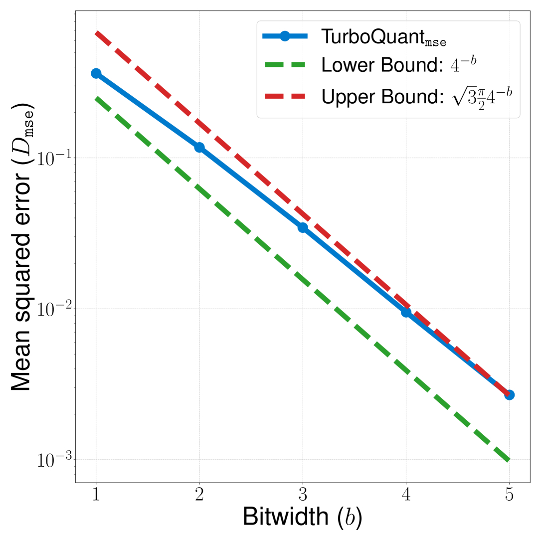 Figure 3b (Zandieh et al., 2025): MSE distortion \(D_{\text{mse}}\) of TurboQuant\(_{\text{mse}}\) (solid blue) plotted against the information-theoretic lower bound \(4^{-b}\) (green dashed) and the theoretical upper bound \(\sqrt{3\pi/2} \cdot 4^{-b}\) (red dashed) on a log scale. All three scale with the same \(4^{-b}\) exponent, and the actual distortion stays tightly sandwiched within the \(\approx 2.7\times\) gap.
4. TurboQuantprod: Unbiased Inner Product Quantization
4.1 Bias of MSE Quantizers
MSE-optimal quantizers are not unbiased for inner products. Consider \(b=1\): the optimal 1-bit MSE codebook for coordinates of a unit sphere consists of \(\pm\sqrt{2/(\pi d)}\). This means \(Q_{\text{mse}}(x) = \text{sign}(\Pi x)\) and the dequantization map is \(Q_{\text{mse}}^{-1}(z) = \sqrt{2/(\pi d)} \cdot \Pi^\top z\). Then:
\[\mathbb{E}[\langle y, Q_{\text{mse}}^{-1}(Q_{\text{mse}}(x))\rangle] = \frac{2}{\pi} \langle y, x\rangle \neq \langle y, x\rangle.\]
The bias is \(2/\pi \approx 0.637\), a significant multiplicative error. This bias decreases as \(b\) increases (the MSE quantizer converges to identity), but is present for all finite \(b\).
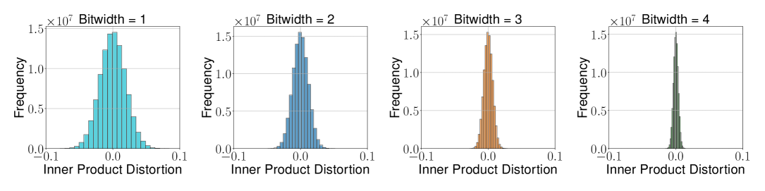 Figure 1a (Zandieh et al., 2025): Inner product distortion histogram for TurboQuant\(_{\text{prod}}\) at bit-widths \(b=1,2,3,4\). The distribution is symmetric and centered at zero, confirming the unbiasedness of the two-stage scheme.
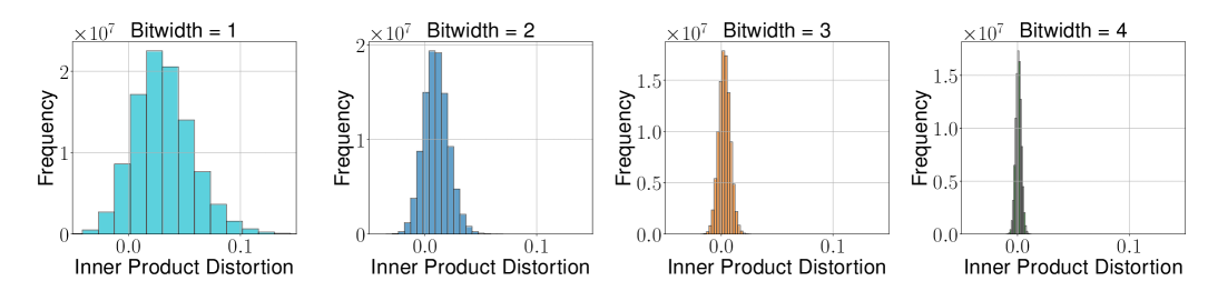 Figure 1b (Zandieh et al., 2025): Inner product distortion histogram for TurboQuant\(_{\text{mse}}\) at the same bit-widths. The distribution is visibly skewed with a non-zero mean, showing the systematic bias of the MSE-optimal quantizer when used for inner product estimation.
In nearest-neighbor search, a biased estimator would score all database points systematically low relative to the true inner products, distorting rankings and reducing recall. In KV cache quantization, a multiplicative bias on attention logits directly distorts attention weights and degrades generation quality.
4.2 Two-Stage QJL Residual Scheme
The fix: compose \(Q_{\text{mse}}\) at bit-width \(b-1\) with a QJL 1-bit sketch on the residual.
Let \(r := x - Q_{\text{mse}}^{-1}(Q_{\text{mse}}(x))\) be the quantization residual. Define
\[Q_{\text{prod}}(x) := \bigl(Q_{\text{mse}}(x),\; Q_{\text{qjl}}(r),\; \|r\|_2\bigr),\]
where \(Q_{\text{qjl}}\) is a QJL sketch matrix \(S \in \mathbb{R}^{d \times d}\) followed by sign-bit quantization. Dequantization:
\[Q_{\text{prod}}^{-1}(\cdot) = Q_{\text{mse}}^{-1}(Q_{\text{mse}}(x)) + \|r\|_2 \cdot Q_{\text{qjl}}^{-1}(Q_{\text{qjl}}(r)),\]
where the QJL dequantization is the QJL asymmetric inner product estimator.
def turbo_quant_prod(x, codebook_b_minus_1, S):
"""Two-stage: MSE quantizer at (b-1) bits + QJL on residual."""
# Stage 1: MSE quantization at (b-1) bits
idx_mse = quantize(x, codebook_b_minus_1) # d × (b-1) bits
x_mse = dequantize(idx_mse, codebook_b_minus_1)
# Stage 2: QJL on residual
r = x - x_mse
gamma = np.linalg.norm(r) # 1 FP16 scalar
qjl_bits = np.sign(S @ r) # d × 1 bits
return idx_mse, qjl_bits, gamma
def inner_product_estimate(y, idx_mse, qjl_bits, gamma, codebook, S):
x_mse = dequantize(idx_mse, codebook)
qjl_estimate = (np.sqrt(np.pi / 2) / len(qjl_bits)) * gamma * np.dot(S @ y, qjl_bits)
return np.dot(y, x_mse) + qjl_estimate # unbiased!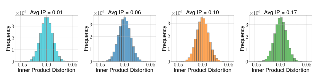 Figure 2a (Zandieh et al., 2025): Inner product error distribution for TurboQuant\(_{\text{prod}}\) conditioned on different average inner product values (b=2). The spread remains constant regardless of the average IP, confirming homoskedasticity.
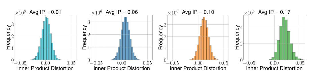 Figure 2b (Zandieh et al., 2025): Inner product error distribution for TurboQuant\(_{\text{mse}}\) at the same settings. The variance grows with the average inner product — a direct consequence of the multiplicative bias: the error \(\langle y,x\rangle(1 - 2/\pi)\) scales with the true inner product.
4.3 Inner Product Distortion Bound (Theorem 2)
🔑 Theorem 2. \(Q_{\text{prod}}\) at bit-width \(b\) satisfies, for any \(x \in S^{d-1}\) and any \(y\):
Unbiasedness: \(\mathbb{E}[\langle y, Q_{\text{prod}}^{-1}(Q_{\text{prod}}(x))\rangle] = \langle y, x\rangle\).
Distortion: \(D_{\text{prod}} \leq \dfrac{3\pi^2 \|y\|_2^2}{d} \cdot \dfrac{1}{4^b}\).
For \(b = 1,2,3,4\): \(D_{\text{prod}} \approx 1.57/d,\; 0.56/d,\; 0.18/d,\; 0.047/d\).
📐 Proof sketch. Let \(\tilde{x}_{\text{mse}} = Q_{\text{mse}}^{-1}(Q_{\text{mse}}(x))\) and \(r = x - \tilde{x}_{\text{mse}}\).
Unbiasedness: By law of total expectation and linearity,
\[\mathbb{E}[\langle y, \hat{x}\rangle \mid \tilde{x}_{\text{mse}}] = \langle y, \tilde{x}_{\text{mse}}\rangle + \mathbb{E}[\langle y, \hat{x}_{\text{qjl}}\rangle \mid \tilde{x}_{\text{mse}}] = \langle y, \tilde{x}_{\text{mse}}\rangle + \langle y, r\rangle = \langle y, x\rangle,\]
using QJL unbiasedness for the middle step. Taking the outer expectation gives unbiasedness.
Distortion: Conditioning on \(\tilde{x}_{\text{mse}}\) and applying the QJL variance bound (Lemma 3.5 of QJL):
\[\mathbb{E}\bigl[|\langle y, x\rangle - \langle y, \hat{x}\rangle|^2 \mid \tilde{x}_{\text{mse}}\bigr] = \text{Var}[\langle y, \hat{x}_{\text{qjl}}\rangle] \leq \frac{\pi}{2d} \|r\|_2^2 \|y\|_2^2.\]
Averaging over \(\tilde{x}_{\text{mse}}\) and applying Theorem 1 at bit-width \(b-1\):
\[D_{\text{prod}} \leq \frac{\pi \|y\|_2^2}{2d} \cdot D_{\text{mse}}(b-1) \leq \frac{\pi \|y\|_2^2}{2d} \cdot \frac{2\sqrt{3\pi}}{4^{b-1}} = \frac{3\pi^2 \|y\|_2^2}{d} \cdot \frac{1}{4^b}. \quad \square\]
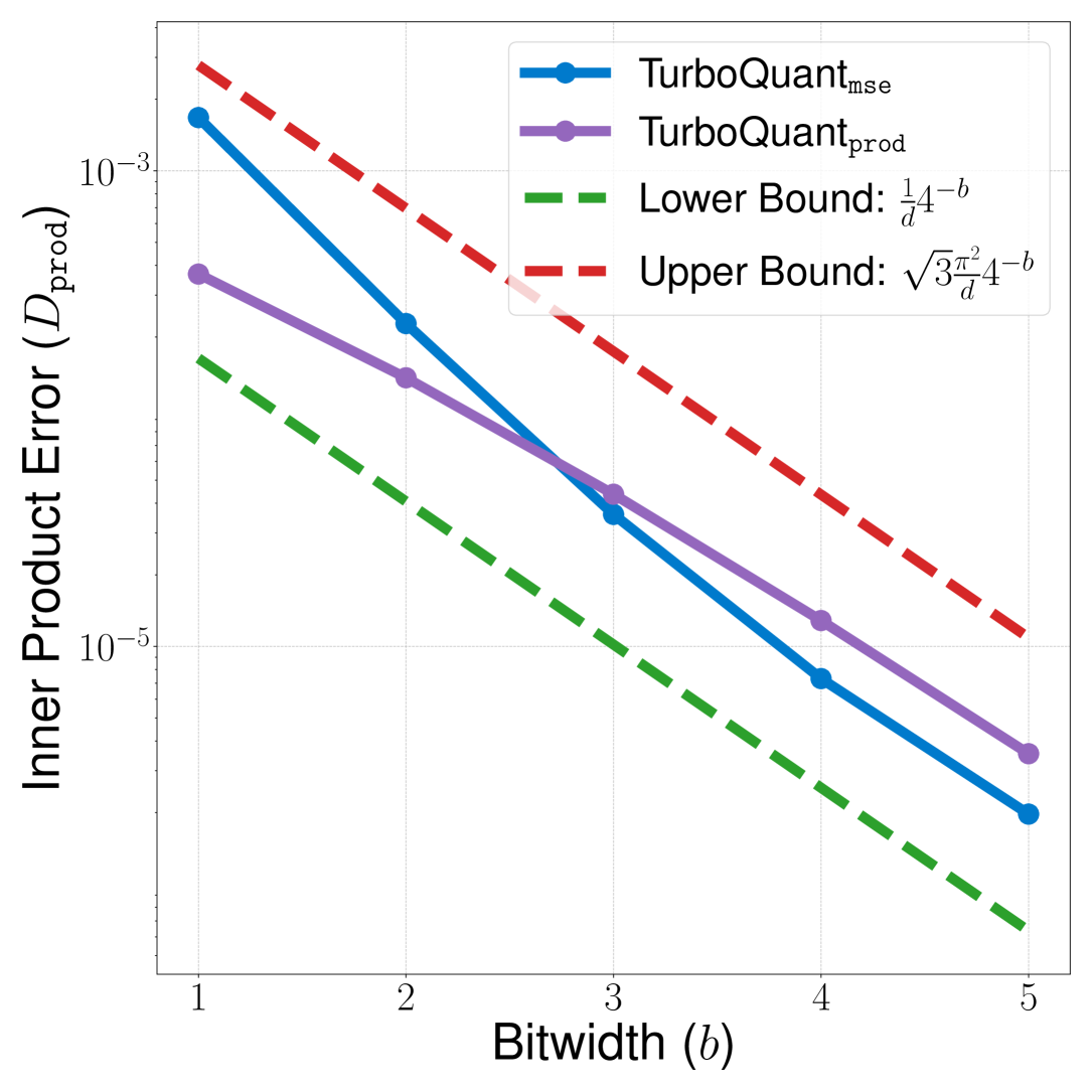 Figure 3a (Zandieh et al., 2025): Inner product error \(D_{\text{prod}}\) vs bit-width \(b\) for TurboQuant\(_{\text{prod}}\) (purple) and TurboQuant\(_{\text{mse}}\) (blue), plotted against the information-theoretic lower bound \(\frac{1}{d}4^{-b}\) (green dashed) and the theoretical upper bound \(\frac{\sqrt{3}\pi^2}{d}4^{-b}\) (red dashed). TurboQuant\(_{\text{prod}}\) consistently outperforms the unbiased-but-lossy MSE approach at all bit-widths, and both track the \(4^{-b}\) scaling law.
5. Experiments
All experiments on a single NVIDIA A100 GPU.
KV Cache Quantization (Llama-3.1 and Llama-3.2 families):
| Method | Bits | Quality |
|---|---|---|
| FP16 (exact) | 16 | Neutral baseline |
| TurboQuant\(_{\text{prod}}\) | 3.5 | Absolute quality neutrality |
| TurboQuant\(_{\text{prod}}\) | 2.5 | Marginal quality degradation |
Nearest Neighbor Search (DBpedia, 1536-dim OpenAI embeddings):
- At the same bit budget, TurboQuant\(_{\text{prod}}\) outperforms product quantization (PQ) and ScaNN variants in recall@1.
- Indexing time is virtually zero (no offline \(k\)-means training required) vs. hours for PQ.
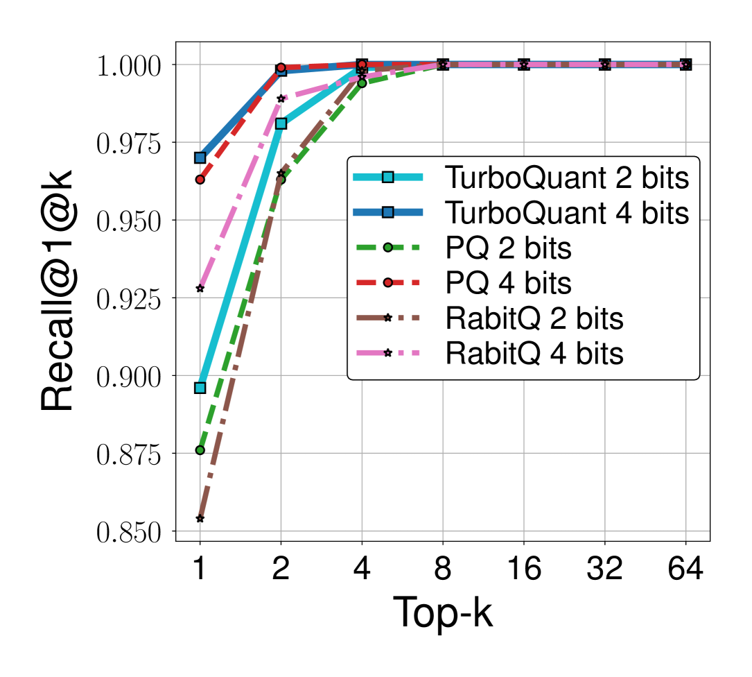 Figure 5b (Zandieh et al., 2025): Recall@1 at top-\(k\) on OpenAI 1536-dimensional embeddings. TurboQuant at 2 bits matches or exceeds PQ and RabitQ at 2 bits across all values of \(k\), and at 4 bits it converges to near-perfect recall at \(k=4\). Crucially, TurboQuant requires no offline training while PQ requires expensive \(k\)-means clustering.
The paper verifies that after random rotation, the coordinate histogram of actual LLM key embeddings matches the predicted Beta distribution closely. This confirms that the theoretical analysis — designed for worst-case unit sphere vectors — accurately predicts behavior on real LLM activations.
6. References
| Reference | Brief Summary | Link |
|---|---|---|
| Zandieh et al. (TurboQuant, 2025) | This paper | arXiv:2504.19874 |
| Zandieh et al. (QJL, 2024) | 1-bit JL quantizer used as subroutine | arXiv:2406.03482 |
| Shannon (1948, 1959) | Source coding and rate-distortion theory | Classic |
| Zador (1963) | High-resolution VQ distortion-rate theory | Paper |
| Lloyd (1982), Max (1960) | Scalar quantizer optimization (Lloyd-Max algorithm) | Classic |
| Gersho (1979) | Vector quantization theory and Gersho’s conjecture | Paper |
| Han et al. (PolarQuant, 2025) | Parallel work using random preconditioning + polar transform | arXiv:2502.02617 |